Chapter 3 - A review of one-phase mantle dynamics¶

%matplotlib inline
from matplotlib import pyplot as plt
import numpy as np 

import warnings 
warnings.filterwarnings('ignore') 

Kinematic solutions for corner flow¶

We consider the incompressible, isoviscous, dimensional Stokes equations without body forces,

\[\begin{align*} \boldsymbol{\nabla} P - \eta\nabla^2\boldsymbol{v} & = \boldsymbol{0},\\ \boldsymbol{\nabla}\!\cdot\boldsymbol{v} & = 0. \end{align*}\]

Under the assumptions described in Section 3.3, we obtain the biharmonic equation,

\[\begin{equation*} \nabla^2(\nabla^2\psi) = 0. \end{equation*}\]

We wish to solve this equation in the wedge-shaped region below the sloping base of the lithospheric plates.

In 2-D polar coordinates, the biharmonic equation (not shown) has the simple, separable solution

\[\begin{split} \begin{align} \label{eq:one-phase-biharm-solution-general} \psi &= rU_0f(\theta), \\ \label{eq:vel-polar} \boldsymbol{v} &= U_0\left[f'(\theta)\rhat - f(\theta)\thetahat\right],\\ \label{eq:pres-polar} P &= -\frac{\eta U_0}{r}\left[f'''(\theta) + f'(\theta)\right], \end{align} \end{split}\]

with

\[ \begin{equation} \label{eq:one-phase-biharm-solution-thetadep} f(\theta) = C_1\sin\theta + C_2\theta\sin\theta + C_3\cos\theta + C_4\theta\cos\theta. \end{equation} \]

Assuming that the lithospheric plates move horizontally away from the ridge axis at speed \(U_0\), we obtain

\[ \begin{equation} \label{eq:one-phase-cornerflow-constants} C_1 = \frac{2\sin^2\theta}{\pi-2\theta-\sin2\theta},\;\;\; C_2 = C_3 = 0,\;\;\; C_4 = \frac{-2}{\pi-2\theta-\sin2\theta}. \end{equation} \]

Combining \(\eqref{eq:one-phase-cornerflow-constants}\) and \(\eqref{eq:one-phase-biharm-solution-thetadep}\), with \(\eqref{eq:vel-polar}\) and \(\eqref{eq:pres-polar}\) gives the solution

\[\begin{split} \begin{align} \label{eq:one-phase-cornerflow-vel} \boldsymbol{v} &= U_0\left\{\left[(C_1+C_4)\cos\theta - C_4\theta\sin\theta\right]\rhat - (C_1\sin\theta + C_4\theta\cos\theta)\thetahat\right\},\\ \label{eq:one-phase-cornerflow-press} P &= \frac{2\eta U_0}{r}C_4\cos\theta. \end{align} \end{split}\]

The Python implementation of equations \(\eqref{eq:one-phase-cornerflow-vel}\) and \(\eqref{eq:one-phase-cornerflow-press}\) are shown below:

def solution_polar_coords(X, Z, theta):

    R = np.sqrt(X ** 2 + Z ** 2)
    T = np.arctan2(X, -Z)
    C1 = 2. * np.sin(theta) ** 2 / (np.pi - 2. * theta - np.sin(2. * theta))
    C4 = -2. / (np.pi - 2. * theta - np.sin(2. * theta))
    vr = (C1 + C4) * np.cos(T) - C4 * T * np.sin(T)
    vt = -(C1 * np.sin(T) + C4 * T * np.cos(T))
    U = vr * np.sin(T) + vt * np.cos(T)
    W = -vr * np.cos(T) + vt * np.sin(T)
    P = 2. * C4 / R * np.cos(T)
    P = np.asarray([
        [p if np.abs(t) <= 0.5 * np.pi - theta else np.NaN for t, p in zip(rT, rP)] 
        for rT, rP in zip(T, P)
    ])

    return U, W, P

Expressing these results in the Cartesian coordinate system, we obtain

\[\begin{split} \begin{align} \label{eq:one-phase-cornerflow-cartesian-vel-x} \boldsymbol{v}\cdot\hat{\boldsymbol{x}} &= U_0C_4\left(\arctan\frac{x}{z} - \frac{xz}{x^2 + z^2}\right), \\ \label{eq:one-phase-cornerflow-cartesian-vel-z} \boldsymbol{v}\cdot\hat{\boldsymbol{z}} &= U_0C_4\left(\sin^2\theta_p - \frac{z^2}{x^2 + z^2}\right), \\ \label{eq:one-phase-cornerflow-cartesian-press} P &= 2\eta U_0 C_4 \frac{-z}{x^2 + z^2}. \end{align} \end{split}\]

The Python implementation of equations \(\eqref{eq:one-phase-cornerflow-cartesian-vel-x}\)-\(\eqref {eq:one-phase-cornerflow-cartesian-press}\) are shown below:

def solution_cartesian_coords(X, Z, theta):

    C1 = 2. * (np.sin(theta)) ** 2 / (np.pi - 2. * theta - np.sin(2. * theta))
    C4 = -2. / (np.pi - 2. * theta - np.sin(2. * theta))
    T = -np.arctan(X/Z)
    Q = (X ** 2 + Z ** 2)

    U = C4 * (np.arctan(X/Z) - X * Z / Q)
    W = C4 * (np.sin(theta) ** 2 - Z ** 2. / Q)
    P = -2. * C4 * Z / Q

    P = np.asarray([
        [p if np.abs(t) <= 0.5 * np.pi - theta else np.NaN for t, p in zip(rT, rP)]
        for rT, rP in zip(T, P)
    ])

    return U, W, P

This notebook exemplifies the corner flow model with the dip of the lithosphere base \(\theta_p\), which physically varies from \(0^\circ\) to nearly \(60^\circ\):

theta_p = 25. * np.pi / 180.  # it can vary from 0 to 60 deg.

The velocity and pressure from \(\eqref{eq:one-phase-cornerflow-vel}\) and \(\eqref{eq:one-phase-cornerflow-press}\) (or, equivalently, \(\eqref{eq:one-phase-cornerflow-cartesian-vel-x}\)-\(\eqref{eq:one-phase-cornerflow-cartesian-press}\)) are computed below:

x = np.linspace(-1.0, 1.0, 500)
z = np.linspace(-1.0, 0.0, 500)

[X, Z] = np.meshgrid(x, z)

# switch between polar and cartesian coordinate system:
# [U, W, P] = solution_polar_coords(X, Z, theta_p)  # refer to equations (6) and (7) 
[U, W, P] = solution_cartesian_coords(X, Z, theta_p);  # reter to equations (8) and (10)

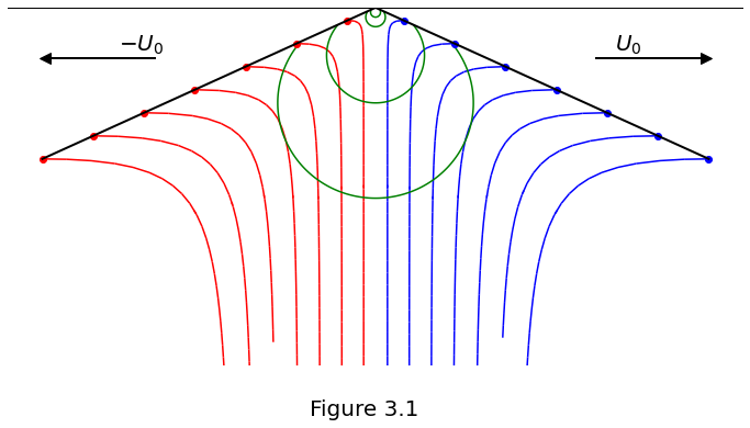
Figure 3.1 plots the velocity streamlines and pressure contours.

fig, ax = plt.subplots()
fig.set_size_inches(12., 6.)

nlines = 7
sm = 0.2 * np.minimum(np.sin(theta_p), np.cos(theta_p))

# velocity streamlines in the positive X axis
seed = np.zeros([nlines, 2])
seed[:, 0] = np.linspace(sm*np.cos(theta_p), np.cos(theta_p), nlines)
seed[:, 1] = np.linspace(-sm*np.sin(theta_p), -np.sin(theta_p), nlines)
ax.plot(seed[:, 0], seed[:, 1], 'bo')
ax.streamplot(
    X, Z, U, W, arrowstyle='-', color='b', start_points=seed, 
    integration_direction='backward'
)

# velocity streamlines in the negative X axis
seed[:, 0] = np.linspace(-np.cos(theta_p), -sm*np.cos(theta_p), nlines)
seed[:, 1] = np.linspace(-np.sin(theta_p), -sm*np.sin(theta_p), nlines)
ax.plot(seed[:, 0], seed[:, 1], 'ro')
ax.streamplot(
    X, Z, U, W, arrowstyle='-', color='r', 
    start_points=seed, integration_direction='backward'
)

# pressure contours
ax.contour(
    X, Z, P, levels=[-100., -50., -10., -5.], colors='g', linestyles='-'
)

# plot X axis
ax.plot([-1., 1.], [0., 0.], '-k', linewidth=2)

# plot the bottom of the lithosphere plates
ax.plot(
    [-np.cos(theta_p), 0., np.cos(theta_p)], 
    [-np.sin(theta_p), 0., -np.sin(theta_p)], 
    '-k', linewidth=2
)

# U_0 line
ax.plot([0.6, 0.9], [-np.sin(theta_p)/3., -np.sin(theta_p)/3.], '-k', linewidth=2)
ax.plot(0.9, -np.sin(theta_p)/3., '>k', markersize=10, markerfacecolor='k')
ax.text(0.65, -np.sin(theta_p)/3.5, r'$U_0$', fontsize=20)

# -U_0 line
ax.plot([-0.6, -0.9], [-np.sin(theta_p)/3., -np.sin(theta_p)/3.], '-k', linewidth=2)
ax.plot(-0.9, -np.sin(theta_p)/3., '<k', markersize=10, markerfacecolor='k')
ax.text(-0.7, -np.sin(theta_p)/3.5, r'$-U_0$', fontsize=20)

ax.set_axis_off()

fig.supxlabel("Figure 3.1", fontsize=20)

plt.show()

The Dynamics of Partially Molten Rock

Chapter 3 - A review of one-phase mantle dynamics¶

Kinematic solutions for corner flow¶