Chapter 7 - Porosity-band emergence under deformation
%matplotlib inline
import matplotlib.pyplot as plt
import numpy as np
from scipy import integrate
from scipy.interpolate import griddata
The (in)stability of perturbations
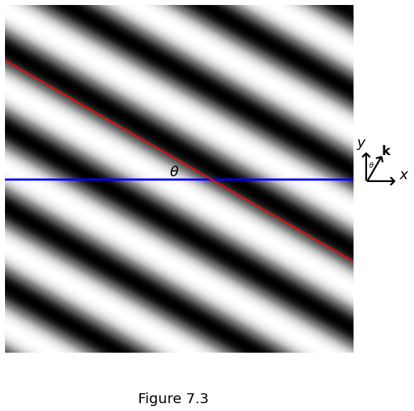
Our perturbation will take the form of harmonic plane waves,
The orientation of these waves is described by an angle \(\theta\) to the \(x\)-axis, as shown in the Figure 7.3 below.
theta = 30.
fig, ax = plt.subplots()
fig.set_size_inches(9., 9.)

x = np.linspace(-1., 1., 1000)
y = np.linspace(-1., 1., 1000)
[X, Y] = np.meshgrid(x,y)

k0 = 3. * 2. * np.pi
theta_rad = theta * np.pi/180.
k = np.asarray([k0 * np.sin(-theta_rad), k0 * np.cos(-theta_rad)])
z = np.real(np.exp(1.j * (k[0] * X + k[1] * Y)))

ax.imshow(z, extent=[-1.5, 1.1, -1.5, 1.1], cmap=plt.get_cmap('Greys'))
ax.set_xlim(-1.1, 1.1)
ax.set_ylim(-1.1, 1.1)

ax.plot([-1.1, 1.1], [0., 0.], '-b', linewidth=3)
ax.plot(
    [0.2, 0.2 - 2. * np.cos(theta_rad)],
    [0., 2. * np.sin(theta_rad)],
    '-r', linewidth=2
)
ax.plot(
    [0.2, 0.2 + 2. * np.cos(theta_rad)],
    [0., -2. * np.sin(theta_rad)],
    '-r', linewidth=2
)

ax.text(0., 0., r'$\theta$', fontsize=20, ha='right', va='bottom')
ax.text(1.15, -0.05, r'$\longrightarrow$', fontsize=30)
ax.text(1.39, 0., r'$x$', fontsize=20)
ax.text(1.12, -0.015, r'$\longrightarrow$', fontsize=30, rotation=90)
ax.text(1.12, 0.2, r'$y$', fontsize=20)
ax.text(1.12, -0.045, r'$\longrightarrow$', fontsize=30, rotation=90-theta)
ax.text(1.28, 0.15, r'$\mathbf{k}$', fontsize=18)
ax.text(1.195, 0.07, r'$\theta$', fontsize=10)

fig.supxlabel("Figure 7.3", fontsize=20)

ax.set_axis_off()
plt.show()
Pure shear
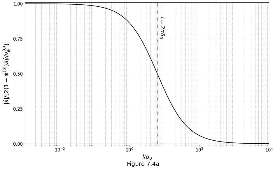
The dispersion relation is
Dispersion curves showing normalised growth rate of perturbations versus perturbation wavelength are plotted in Figure 7.4a below on log-linear axes:
fig, ax = plt.subplots()
fig.set_size_inches(15., 9.)

x = 2. * np.pi * np.logspace(-6., 4., 1000)
y = (2. * np.pi  / x) / (1. + 2. * np.pi / x)

ax.semilogx(x, y, '-k', linewidth=2)
ax.set_xlim(1e-3, 1e4)
ax.set_ylim(-0.01, 1.01)

ax.plot([2. * np.pi, 2. * np.pi], [-0.01, 1.01], ':r')
ax.text(
    2. * np.pi * 1.1, 0.75, r'$l=2\pi\delta_{0}$',
    rotation=-90, va='bottom', fontsize=20
)
ax.set_xlabel(r'$l/\delta_{0}$', fontsize=20)
ax.set_xticks((1e-2, 1e0, 1e2, 1e4))
plt.gca().xaxis.grid(True, which='minor', linestyle='--')
ax.set_ylabel(
    r'$\vert \dot{s}\vert/[2(1-\phi^{(0)})\lambda\dot{\gamma}/\nu^{(0)}_\phi]$',
    fontsize=20
)
ax.set_yticks((0.0, 0.25, 0.5, 0.75, 1.))
ax.tick_params(axis='both', which='major', labelsize=15)
plt.gca().yaxis.grid(True, which='major')

fig.supxlabel("Figure 7.4a", fontsize=20)

plt.show()
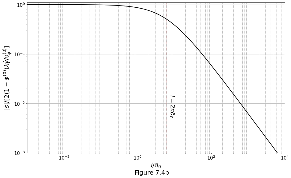
and on log-log axes in Figure 7.4b:
fig, ax = plt.subplots()
fig.set_size_inches(15.0, 9.0)

x = 2. * np.pi * np.logspace(-6.0, 4.0, 1000)
y = (2. * np.pi / x)/(1. + 2. * np.pi / x)

ax.loglog(x, y, '-k', linewidth=2)
ax.set_xlim(1e-3, 1e4)
ax.set_ylim(1e-3, 1.1)

ax.set_xlabel(r'$l/\delta_{0}$', fontsize=20)
ax.set_xticks((1e-2, 1e0, 1e2, 1e4))
plt.gca().xaxis.grid(True, which='minor', linestyle='--')
ax.set_ylabel(
    r'$\vert \dot{s}\vert/[2(1-\phi^{(0)})\lambda\dot{\gamma}/\nu^{(0)}_\phi]$',
    fontsize=20
)
ax.set_yticks((1e-3, 1e-2, 1e-1, 1e0))
plt.gca().yaxis.grid(True, which='major')

ax.plot([2.*np.pi, 2.*np.pi], [1e-10, 10.0], ':r')
ax.text(
    2. * np.pi * 1.1, 0.005, r'$l=2\pi\delta_{0}$',
    rotation=-90, va='bottom', fontsize=20
)
ax.tick_params(axis='both', which='major', labelsize=15)

fig.supxlabel("Figure 7.4b", fontsize=20)

plt.show()
Simple shear
Porosity advection by the base-state
Figure 7.5a plots the schematic diagram normal to the shear plane showing a representative high-porosity band oriented at an angle \(\theta\) with normal \(\boldsymbol{k}\). The band is being rotated to higher \(\theta\) by the simple-shear flow.
th2 = 20.0
fig, ax = plt.subplots()
fig.set_size_inches(6., 6.)

rot = -th2*np.pi/180.
M = np.asarray(((np.cos(rot), -np.sin(rot)), (np.sin(rot), np.cos(rot))))
aM = np.dot(M, np.asarray(((-1., 1.), (0.0, 0.0))))
ax.plot(aM[0, :], aM[1, :], '-k', linewidth=3)
ax.plot([-1., 1.], [-np.sin(rot), -np.sin(rot)], 'k')  # bottom line
ax.plot([-1., 1.], [0., 0.], '--k')  # middle line
ax.plot([-1., 1.], [np.sin(rot), np.sin(rot)], 'k')  # top line
ax.plot(
    [-0.3, 0.3, 0.1], [1.1*np.sin(rot),
    1.1*np.sin(rot), 1.2*np.sin(rot)], 'r'
)  # top red arrow
ax.plot(
    [0.3, -0.3, -0.1],
    [-1.1*np.sin(rot), -1.1*np.sin(rot), -1.2*np.sin(rot)],
    'r'
)  # bottom red arrow

al = 0.5 * np.abs(np.sin(rot))
ahl = 0.05 * np.abs(np.sin(rot))
av = np.zeros(5 * 2).reshape(2, 5)
av[0, :] = np.asarray((0., al, al-ahl, al, al-ahl))
av[1, :] = np.asarray((0., 0., ahl, 0., -ahl))
rot_90 = (90.-th2)*np.pi/180.
M = np.asarray((
    (np.cos(rot_90), -np.sin(rot_90)),
    (np.sin(rot_90),  np.cos(rot_90))
))
aM = np.dot(M, av)
ax.plot(aM[0, :], aM[1, :], '-k')
ax.text(aM[0, -1], aM[1, -1], r'$\mathbf{k}$', fontsize=20, va='top', ha='left')

ax.set_xlim(-1.0, 1.0)
ax.set_ylim(-1.0, 1.0)
ax.text(
    -0.5 * np.abs(np.cos((180. - th2) * np.pi / 180.)),
    0.04, r'$\theta$', fontsize=20
)
ax.text(0.4, 0.05, r'shear plane', fontsize=20)

fig.supxlabel("Figure 7.5a", fontsize=20)

ax.set_axis_off()
plt.show()
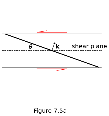
Figure 7.5a above shows a wave-front with wavevector \(\boldsymbol{k}\) at time \(t\). It makes an angle to the shear plane of
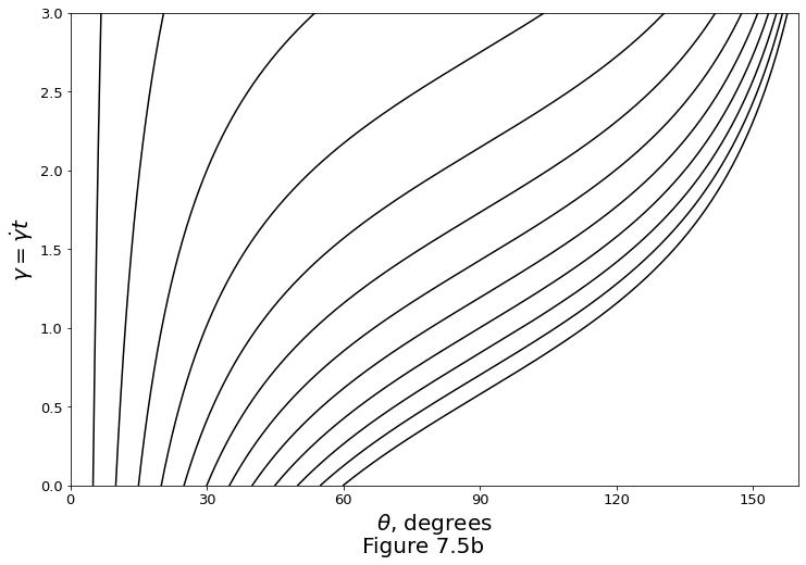
A plot of band angle from equation \(\eqref{eq:simpleshear-bandangle}\) as a function of progressive shear strain (on the \(y\)-axis) is shown in Figure 7.5b below.
fig, ax = plt.subplots()
fig.set_size_inches(12., 8.)

th0 = np.arange(5, 61, 5)*np.pi/180.
t = np.linspace(0., 3., 1000)
th = np.asarray(
    [np.arctan2(np.sin(th0i), np.cos(th0i) - t*np.sin(th0i)) for th0i in th0]
)

for th_ in th:
    ax.plot(th_*180/np.pi, t, '-k')
ax.set_xlim(0., 160.)
ax.set_ylim(0., 3.)
ax.set_xlabel(r'$\theta$, degrees', fontsize=20)
ax.set_xticks(np.arange(0.0, 150.1, 30.0))
ax.set_ylabel(r'$\gamma = \dot{\gamma}t$', fontsize=20)
ax.set_yticks((0.0, 0.5, 1, 1.5, 2, 2.5, 3))
ax.tick_params(axis='both', which='major', labelsize=13)

fig.supxlabel("Figure 7.5b", fontsize=20)

plt.show()
Growth of porosity bands when \(\mathfrak{n}=1\)
The growth rate can be written as
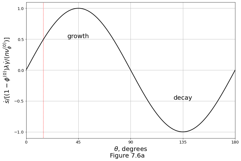
Figure 7.6a below plots the normalised growth rate of small-wavelength (\(l\ll\delta_0\)) porosity bands under simple shear and Newtonian viscosity.
fig, ax = plt.subplots()
fig.set_size_inches(12., 8.)

theta = np.linspace(0., np.pi, 1000)

ax.plot([15., 15.], [-2., 2.],':r')
ax.plot(theta*180./np.pi, np.sin(2.*theta), '-k', linewidth=2)
ax.set_xlim(0., 180.)
ax.set_ylim(-1.1, 1.1)

ax.set_xlabel(r'$\theta$, degrees', fontsize=20)
ax.set_xticks(np.arange(0.0, 180.1, 45.))
ax.set_ylabel(
    r'$\dot{s}/[(1-\phi^{(0)})\lambda\dot{\gamma}/(n\nu^{(0)}_\phi)]$',
    fontsize=20
)
ax.set_yticks(np.arange(-1.0, 1.01, 0.5))
ax.text(45., 0.5, 'growth', fontsize=20, ha='center', va='bottom')
ax.text(135., -0.5, 'decay', fontsize=20, ha='center', va='bottom')
ax.tick_params(axis='both', which='major', labelsize=13)
plt.grid(True)

fig.supxlabel("Figure 7.6a", fontsize=20)

plt.show()
Growth of porosity bands when \(\mathfrak{n} \ge 1\)
The growth rate can be written as
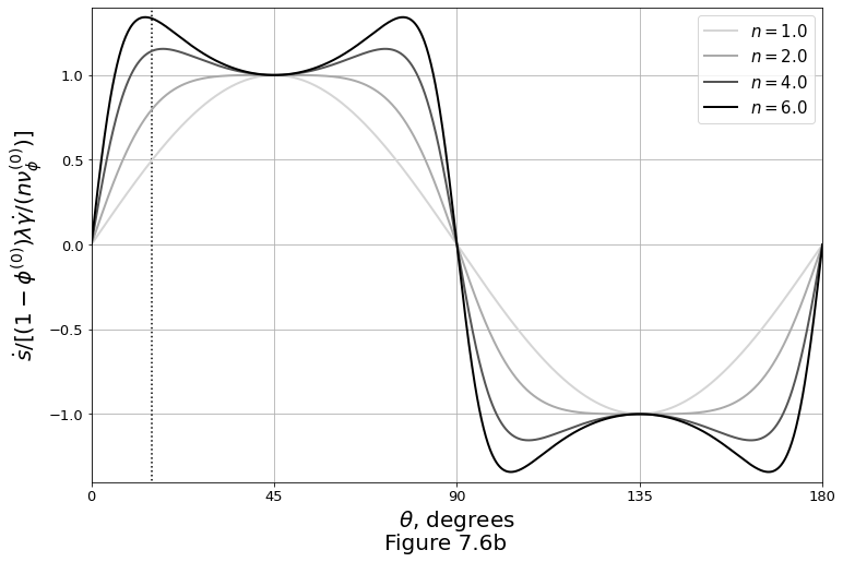
Figure 7.6b below plots the normalised growth rate of small-wavelength (\(l\ll\delta_0\)) porosity bands under simple shear and non-Newtonian viscosity with various values of \(\mathfrak{n}\). The vertical dotted lines mark \(\theta=15^\circ\).
fig, ax = plt.subplots()
fig.set_size_inches(12., 8.)

ax.plot([15., 15.], [-2., 2.], ':k')
n = np.asarray((1., 2., 4., 6.))
theta = np.linspace(0., np.pi, 1000)
for i in n:
    N = (i - 1.)/i
    colr = [
        1. - i/np.amax(n), 1. - i/np.amax(n), 1. - i/np.amax(n)
    ]
    ax.plot(
        theta*180./np.pi, np.sin(2.*theta)/(1.-N*np.cos(2.*theta)**2),
        linewidth=2, label=r'$n='+str(i)+'$', color=colr
    )

ax.set_xlim(0., 180.)
ax.set_ylim(-1.4, 1.4)
ax.set_xlabel(r'$\theta$, degrees', fontsize=20)
ax.set_xticks(np.arange(0.0, 180.1, 45.))
ax.set_ylabel(
    r'$\dot{s}/[(1-\phi^{(0)})\lambda\dot{\gamma}/(n\nu^{(0)}_\phi)]$',
    fontsize=20
)
ax.set_yticks(np.arange(-1.0, 1.01, 0.5))
ax.legend(fontsize=15, loc='upper right')
ax.tick_params(axis='both', which='major', labelsize=13)
plt.grid(True)

fig.supxlabel("Figure 7.6b", fontsize=20)

plt.show()
Extending the analysis to finite strain
Restricting our focus to the case of wavelengths much smaller than the compaction length, we can obtain \(s\) by integrating
where \(t'\) is a dummy variable of integration, to distinguish it from the (variable) upper limit of integration, \(t\).
Figure 7.7a below plots the amplitude of porosity perturbations \(\text{e}^{s(t)}\) as a function of angle and strain \(\gamma=\dot{\gamma} t\). Dotted curves are passive advection trajectories from equation \(\eqref{eq:simpleshear-bandangle}\) with Newtonian viscosity (\(\mathfrak{n}=1,\,\mathcal{N}=0\)).
fig, ax = plt.subplots()
fig.set_size_inches(12., 8.)

ncontours = 20

N = 600
tmax = 3.3
th0 = np.linspace(0., 135.*np.pi/180., N, endpoint=True)
t = np.linspace(0., tmax, N)
theta = np.asarray(
    [np.arctan2(np.sin(th0i), np.cos(th0i) - t*np.sin(th0i)) for th0i in th0]
)
amp = np.asarray(
    [integrate.cumtrapz(np.sin(2.*th), t, initial=0) for th in theta]
)

THETA, T = np.meshgrid(th0, t)

tt = np.tile(t, N)
exp_amp = np.exp(amp)
F = griddata(
    (theta.reshape(N*N), tt), exp_amp.reshape(N*N),
    (THETA.reshape(N*N), T.reshape(N*N))
)
A = np.exp(F).reshape(N, N)
A = np.asarray([a/np.max(a) for a in A])

convec = np.linspace(0.05, 0.95, 10, endpoint=True)
convecB = np.linspace(0.05, 0.95, 4, endpoint=True)
convec = np.setdiff1d(convec, convecB)

th0_ = np.concatenate(
    (np.arange(2, 45, 4), np.arange(49, 135, 8)), axis=0
) * np.pi / 180.
th_ = np.asarray(
    [np.arctan2(np.sin(th0i), (np.cos(th0i) - t*np.sin(th0i))) for th0i in th0_]
)

CS = ax.contour(th0*180./np.pi, t, A, convec, cmap=plt.cm.binary, linewidths=1)
CSB = ax.contour(th0*180./np.pi, t, A, convecB, colors='k', linewidths=2)
ax.clabel(CSB, inline=1, fontsize=15)

for thi in th_:
    ax.plot(thi*180./np.pi, t, ':k')
ax.set_xlabel(r'$\theta$, degrees', fontsize=20)
ax.set_ylabel(r'$\gamma=\dot{\gamma}t$', fontsize=20)
ax.set_xlim(0., np.amax(th0_)*180./np.pi)
ax.set_ylim(0., np.amax(t))
ax.set_xticks((0, 15, 30, 45, 60, 90, 120))
ax.set_yticks((0, 1, 2, 3))
ax.tick_params(axis='both', which='major', labelsize=13)

fig.supxlabel("Figure 7.7a", fontsize=20)

plt.show()
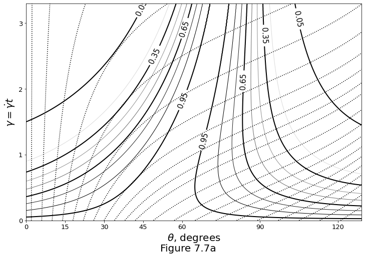
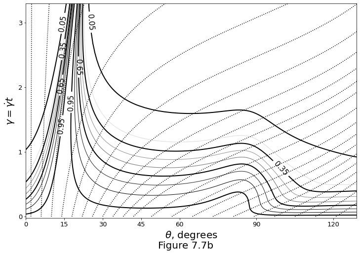
Figure 7.7b below also plots the amplitude of porosity perturbations \(\text{e}^{s(t)}\) as a function of angle and strain \(\gamma=\dot{\gamma} t\), but the dotted curves are passive advection trajectories consider Non-Newtonian viscosity (\(\mathfrak{n}=6,\,\mathcal{N}=5/6\)).
fig, ax = plt.subplots()
fig.set_size_inches(12., 8.)

eps = 2.2204e-16
n = 6.
N = 600
tmax = 3.3
dpts = np.asarray([0., 5., 20., 135.])*np.pi/180.
th0 = np.linspace(dpts[0], dpts[1], int(N/4))
th0 = np.concatenate((th0, np.linspace(dpts[1] + eps, dpts[2], int(N/2))), axis=0)
th0 = np.concatenate((th0, np.linspace(dpts[2] + eps, dpts[3], int(N/4))), axis=0)
assert th0.shape[0] == N, 'th0 was wrongly calculated'

t = np.linspace(0., tmax, N)
nf = (1.-n)/n

theta = np.asarray(
    [np.arctan2(np.sin(th0i), np.cos(th0i) - t*np.sin(th0i)) for th0i in th0]
)
amp = np.asarray([
    integrate.cumtrapz(
        np.sin(2.*th)/(1+nf*np.cos(2.*th)**2), t, initial=0
    ) for th in theta
])

THETA, T = np.meshgrid(th0, t)

tt = np.tile(t, N)
exp_amp = np.exp(amp)
F = griddata(
    (theta.reshape(N*N), tt), exp_amp.reshape(N*N),
    (THETA.reshape(N*N), T.reshape(N*N))
)
A = np.exp(F).reshape(N, N)
A = np.asarray([a/np.max(a) for a in A])

convec = np.linspace(0.05, 0.95, 10, endpoint=True)
convecB = np.linspace(0.05, 0.95, 4, endpoint=True)
convec = np.setdiff1d(convec, convecB)

th0_ = np.concatenate(
    (np.arange(2, 45, 4), np.arange(49, 135, 8)), axis=0
) * np.pi / 180.

th = np.asarray(
    [np.arctan2(np.sin(th0i), np.cos(th0i) - t*np.sin(th0i)) for th0i in th0_]
)

CS = ax.contour(th0*180./np.pi, t, A, convec, cmap=plt.cm.binary, linewidths=1.0)
CSB = ax.contour(th0*180./np.pi, t, A, convecB, colors='k', linewidths=2)
ax.clabel(CSB, inline=1, fontsize=15)

for thi in th_:
    ax.plot(thi*180./np.pi, t, ':k')

ax.set_xlabel(r'$\theta$, degrees', fontsize=20)
ax.set_ylabel(r'$\gamma=\dot{\gamma}t$', fontsize=20)
ax.set_xlim(0., np.amax(th0_)*180./np.pi)
ax.set_ylim(-0.02, np.amax(t))
ax.set_xticks((0, 15, 30, 45, 60, 90, 120))
ax.set_yticks((0, 1, 2, 3))
ax.tick_params(axis='both', which='major', labelsize=13)

fig.supxlabel("Figure 7.7b", fontsize=20)

plt.show()
Wavelength selection by surface tension
The growth rate of porosity bands versus wavelength is given by
Increasing values of \(\text{D}_\mathcal{I}\) represent an increasing strength of surface-tension driven segregation. Figure 7.8a below plots \(\eqref{eq:porband-sfcten-growrate-wavenum}\) in log-linear scale.
fig, ax = plt.subplots()
fig.set_size_inches(9., 9.)

k = np.logspace(-2, 3, 10000)
Rb = np.asarray([0., 0.0001, 0.001, 0.01])
sd = np.asarray([k**2.*(1. - Rbi*k**2)/(k**2+1.) for Rbi in Rb])
l_on_d = 2*np.pi/k

for i in np.arange(len(Rb)):
    colr = 1.-(len(Rb) - i)/len(Rb)*np.asarray([1, 1, 1])
    ax.semilogx(
        l_on_d, sd[i, :], '-', linewidth=2,
        color=colr, label=f'$D_I={str(Rb[i])}$'
    )

ax.set_xlabel(r'$l/\delta_{0}$', fontsize=20)
ax.set_xticks(np.power(10., np.arange(-2.0, 2.1, 1.)))
ax.set_xlim(1e-2, np.power(10, 2.8))
plt.gca().xaxis.grid(True, which='minor', linestyle='--')
ax.set_ylabel(
    r'$\dot{s}/[(1-\phi^{(0)})\lambda\dot{\gamma}/(n\nu^{(0)}_\phi)]$',
    fontsize=20
)
ax.set_yticks(np.arange(0., 1.01, 0.25))
ax.set_ylim(-0.02, 1.02)
ax.legend(fontsize=15, loc='upper right')
ax.tick_params(axis='both', which='major', labelsize=13)
plt.grid(True)

fig.supxlabel("Figure 7.8a", fontsize=20)

plt.show()
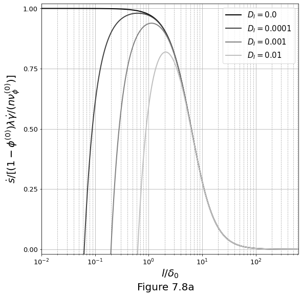
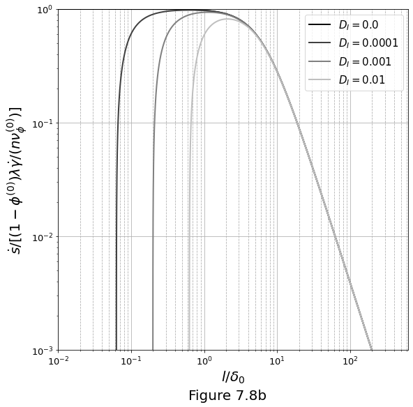
Figure 7.8b below plots \(\eqref{eq:porband-sfcten-growrate-wavenum}\) in the log-log scale.
fig, ax = plt.subplots()
fig.set_size_inches(9., 9.)

k = np.logspace(-2,3,10000)
Rb = np.asarray([0., 0.0001, 0.001, 0.01])
sd = np.asarray([k**2.*(1. - Rbi*k**2)/(k**2+1.) for Rbi in Rb])
l_on_d = 2*np.pi/k

for i in np.arange(len(Rb)):
    colr = 1.-(len(Rb) - i)/len(Rb)*np.asarray([1, 1, 1])
    ax.loglog(
        l_on_d, sd[i, :], '-', linewidth=2,
        color=colr, label=f'$D_I={str(Rb[i])}$'
    )

ax.set_xlabel(r'$l/\delta_{0}$', fontsize=20)
ax.set_xticks(np.power(10., np.arange(-2.0, 2.1, 1.)))
ax.set_xlim(1e-2, np.power(10, 2.8))
plt.gca().xaxis.grid(True, which='minor', linestyle='--')

ax.set_ylabel(
    r'$\dot{s}/[(1-\phi^{(0)})\lambda\dot{\gamma}/(n\nu^{(0)}_\phi)]$',
    fontsize=20
)
ax.set_yticks(np.power(10., np.arange(-3, 0.1, 1)))
ax.set_ylim(1e-3, 1e0)
ax.legend(fontsize=15, loc='upper right')
ax.tick_params(axis='both', which='major', labelsize=13)
plt.grid(True)

fig.supxlabel("Figure 7.8b", fontsize=20)

plt.show()
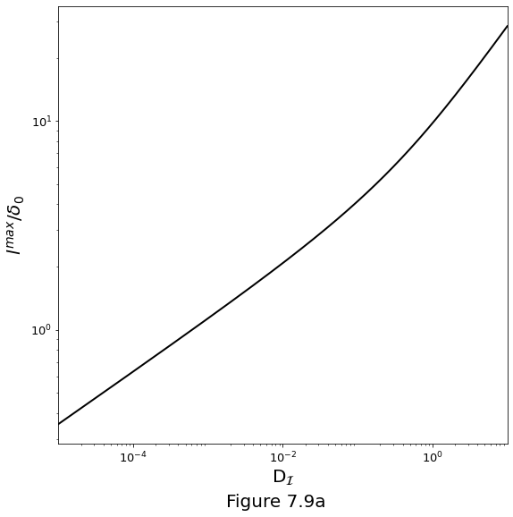
The characteristics of the dominant perturbation as a function of \(\text{D}_\mathcal{I}\) is plotted in Figure 7.9a below for the wavelength with the largest growth rate \(l^\text{max}/\delta_0\).
fig, ax = plt.subplots()
fig.set_size_inches(9., 9.)

Rb = np.logspace(-5., 1., 10000)
ks = np.sqrt((np.sqrt(Rb+1.) - np.sqrt(Rb))/np.sqrt(Rb))
l = 2. * np.pi/ks

ax.loglog(Rb, l, '-k', linewidth=2)
ax.set_xlabel(r'D$_\mathcal{I}$', fontsize=20)
ax.set_xlim(1e-5, 1e1)
ax.set_xticks(np.power(10., np.arange(-4, 1, 2)))
ax.set_ylabel(r'$l^{max}/\delta_{0}$', fontsize=20)
ax.set_yticks((1e0, 1e1))
ax.tick_params(axis='both', which='major', labelsize=13)

fig.supxlabel("Figure 7.9a", fontsize=20)

plt.show()
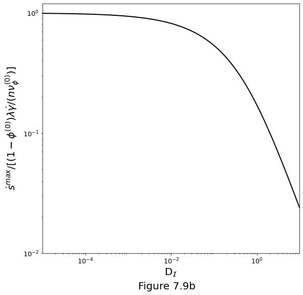
And Figure 7.9b below for the growth rate of the dominant perturbation \(s_*^\text{max}\).
fig, ax = plt.subplots()
fig.set_size_inches(9.0, 9.0)

Rb = np.logspace(-5., 1., 10000)
ks = np.sqrt((np.sqrt(Rb+1.) - np.sqrt(Rb))/np.sqrt(Rb))
s = ks**2. * (1. - Rb*ks**2)/(ks**2. + 1.)

ax.loglog(Rb, s, '-k', linewidth=2)
ax.set_xlim(1e-5, 1e1)
ax.set_xticks(np.power(10., np.arange(-4., 1., 2)))
ax.set_yticks([1e-2, 1e-1, 1e0])
ax.set_xlabel(r'D$_\mathcal{I}$', fontsize=20)
ax.set_ylabel(
    r'$\dot{s}^{max}/[(1-\phi^{(0)})\lambda\dot{\gamma}/(n\nu^{(0)}_\phi)]$',
    fontsize=20
)
ax.tick_params(axis='both', which='major', labelsize=13)

fig.supxlabel("Figure 7.9b", fontsize=20)

plt.show()