Chapter 8 - Conservation of energy
%matplotlib inline
import matplotlib.pyplot as plt
import numpy as np
from scipy.integrate import odeint
Dissipation-driven melting and compaction
The thickness of the layer of ice is the solution of equations
where \(\Pi\), the compaction-dissipation number, is given by
The Python code below implements the right-hand side of equations \(\eqref{eq:cmp-diss-mech-odes-nondim-a}\) and \(\eqref{eq:cmp-diss-mech-odes-nondim-b}\), which will be soon solved numerically.
def thick(y, t, pi, lam):  # y = [H, phi]

    H = y[0]
    phi = y[1]

    return [-pi * H * phi, np.exp(-lam*phi) - pi * (1. - phi) * phi]
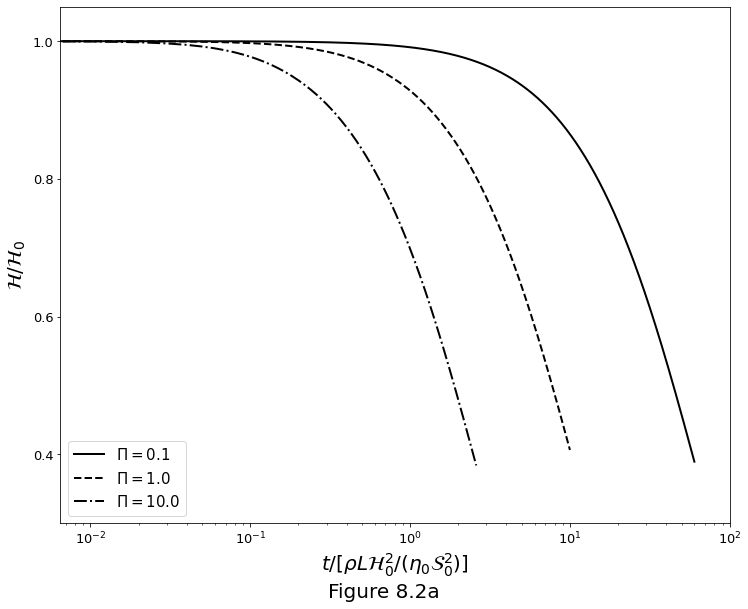
The Figure 8.2a below plots the layer thickness \(\mathcal{H}\) relative to initial versus time for three values of \(\Pi\).
f, ax = plt.subplots()
f.set_size_inches(12., 9.5)

y0 = [1., 0.0]  # initial condition: H=1, phi=0.0
lambda_ = 27.0
Pi = np.asarray([0.1, 1., 10.])
tmax = np.asarray([60., 10., 2.6])
linesty = ['-', '--', '-.']
for tm, pi, ls in zip(tmax, Pi, linesty):
    t = np.arange(0.0, tm, 0.01)
    S = odeint(thick, y0, t, args=(pi, lambda_), rtol=1e-8)
    ax.semilogx(t, S[:, 0], 'k', linestyle=ls, linewidth=2, label=f'$\Pi={str(pi)}$')

ax.set_xlabel(r'$t/[\rho L\mathcal{H}_0^2/(\eta_0\mathcal{S}_0^2)]$', fontsize=20)
ax.set_xticks((1e-2, 1e-1, 1e0, 1e1, 1e2))
ax.set_ylim(0.3, 1.05)
ax.set_ylabel(r'$\mathcal{H}/\mathcal{H}_0$', fontsize=20)
ax.set_yticks((0.4, 0.6, 0.8, 1.0))
ax.legend(loc='lower left', fontsize=15)
ax.tick_params(axis='both', which='major', labelsize=13)

f.supxlabel("Figure 8.2a", fontsize=20)

plt.show()
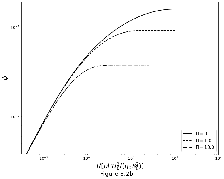
The Figure 8.2b below plots porosity versus time for three values of \(\Pi\).
f, ax = plt.subplots()
f.set_size_inches(12., 9.5)

y0 = [1., 0.0]  # initial condition: H=1, phi=0.0
lambda_ = 27.0
Pi = np.asarray([0.1, 1., 10.])
tmax = np.asarray([60., 10., 2.6])
linesty = ['-', '--', '-.']
for pi, tm, ls in zip(Pi, tmax, linesty):
    t = np.arange(0.0, tm, 0.005)
    S = odeint(thick, y0, t, args=(pi, lambda_), rtol=1e-8)
    ax.loglog(
        t, S[:, 1], 'k', linestyle=ls,
        linewidth=2, label=f'$\Pi={str(pi)}$'
    )

ax.set_xlabel(
    r'$t/[\rho L\mathcal{H}_0^2/(\eta_0\mathcal{S}_0^2)]$',
    fontsize=22
)
ax.set_xticks((1e-2, 1e-1, 1e0, 1e1, 1e2))
ax.set_ylabel(r'$\phi$', fontsize=22)
ax.set_yticks((1e-2, 1e-1))
ax.legend(loc='lower right', fontsize=15)
ax.tick_params(axis='both', which='major', labelsize=13)

f.supxlabel("Figure 8.2b", fontsize=20)

plt.show()
Decompression melting
At depths greater than the onset of decompression melting we have
while within the melting region the isentrope is given by
The Python code below implements the right-hand side of equations \(\eqref{eq:decomp-melting-subsolidus}\) and \(\eqref{eq:decomp-melting-meltregion}\), which will be soon solved numerically.
def TemperatureEquation(T, z, Ts0, rho, g, C, alpha, L, M):

    Tsol = Ts0 - rho*g*z/C

    return -(alpha*T*g/c + rho*g/C)/(1 + L*M/c) if T > Tsol else -alpha*T*g/c
The following constants are defined:
c = 1200.           # heat capacity
alpha = 3e-5        # expansivity
rho = 3000.         # density
g = 10.             # gravity
L = 5e5             # latent heat J/kg
M = 1/500           # isobaric productivity
C = 6.5e6           # clapeyron Pa/K
Ts0 = 1100. + 273.  # solidus at P=0
Tp = 1350. + 273.   # mantle potential temperature
Figure 8.3a below plots the decompression melting curves with no melt segregation. Temperature as a function of \(z\). The solid curve shows the isentropic temperature profile isentrope computed according to equations \(\eqref{eq:decomp-melting-subsolidus}\) and \(\eqref{eq:decomp-melting-meltregion}\). The dashed line shows the isentrope for no melting. Dotted lines are isopleths of the degree of melting \(F\).
f, ax = plt.subplots()
f.set_size_inches(4.5, 9.0)

zF = - (Tp-Ts0)/(rho*g/C - alpha*g*Tp/c)  # metres
zmax = -100.*1000.
Tmax = Tp*np.exp(-alpha*g*zmax/c)

z = np.linspace(zmax, 0., 5000)
T = odeint(
    TemperatureEquation,
    Tmax,
    z,
    args=(Ts0, rho, g, C, alpha, L, M)
)
Tsol = Ts0 - rho*g*z/C

l1 = ax.plot(T-273., z/1000., '-k')[0]
l2 = ax.plot(Tp * np.exp(-alpha*g*z/c) - 273., z/1000., '--k')[0]
for i in [0.0, 0.1, 0.2, 0.3]:
    l3 = ax.plot(Tsol - 273. + i/M, z/1000., ':k')[0]
    ax.text(
        1415, -65+i*110, f'$F={str(i)}$', fontsize=12,
        rotation=-45, horizontalalignment='right'
    )

ax.set_xlabel(r'$T, ^\circ$C', fontsize=20)
ax.set_xticks((1200, 1300, 1400))
ax.set_xlim(1175, 1425)
ax.set_ylabel(r'$z,$ km', fontsize=20)
ax.set_yticks(np.arange(-90., 1., 15))
ax.set_ylim(-99., 0.0)
ax.legend(
    handles=[l1, l2, l3],
    labels=['isentrope', '$\Gamma=0$ isentrope', '$F$ isopleth'],
    loc='lower left', fontsize=12
)
ax.tick_params(axis='both', which='major', labelsize=13)

f.supxlabel("Figure 8.3a", fontsize=20)

plt.show()
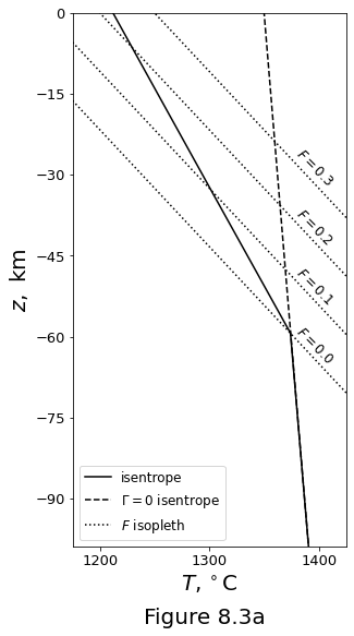
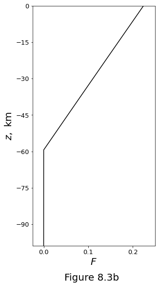
Figure 8.3b plots the degree of melting associated with the isentrope in figure above.
f, ax = plt.subplots()
f.set_size_inches(4.5, 9.0)

zF = - (Tp-Ts0)/(rho*g/C - alpha*g*Tp/c)  # metres
zmax = -100.*1000.
Tmax = Tp*np.exp(-alpha*g*zmax/c)

z = np.linspace(zmax, 0., 5000)
T = odeint(
    TemperatureEquation,
    Tmax,
    z,
    args=(Ts0, rho, g, C, alpha, L, M)
)

Tsol = Ts0 - rho*g*z/C
F = np.maximum(M * (T[:, 0] - Tsol), 0.0)

ax.plot(F, z/1000, '-k')
ax.set_xlabel(r'$F$', fontsize=20)
ax.set_xticks((0.0, 0.1, 0.2, 0.3, 0.4, 0.5))
ax.set_xlim(-0.025, 0.25)
ax.set_ylabel(r'$z,$ km', fontsize=20)
ax.set_yticks(np.arange(-90., 1., 15))
ax.set_ylim(-99., 0.0)
ax.tick_params(axis='both', which='major', labelsize=13)

f.supxlabel("Figure 8.3b", fontsize=20)

plt.show()