Chapter 6 - Compaction and its inherent length scale
The compaction-press problem
%matplotlib inline
import numpy as np
import scipy.sparse as sps
import scipy.sparse.linalg as spla
from scipy.optimize import brentq
import matplotlib.pyplot as plt
from matplotlib import animation
import warnings
warnings.filterwarnings('ignore')
plt.rcParams["animation.html"] = "jshtml"
plt.ioff();
The solution to the Filter Press problem was given as
def compaction_rate(z):
return -np.exp(z)
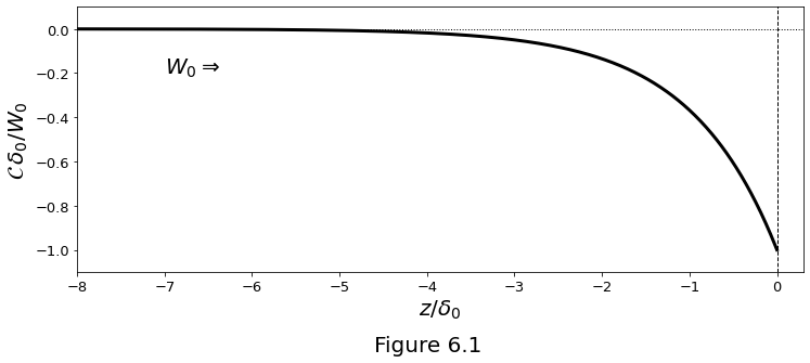
The compact rate function, equation \(\eqref{eq:filterpress-cmprate}\), is plotted in Figure 6.1 below.
fig, ax = plt.subplots()
fig.set_size_inches(12.0, 4.5)
z = np.linspace(-8, 0.0, 1000)
C = compaction_rate(z)
ax.plot([0., 0], [-2., 2], '--k', linewidth=1)
ax.plot([-8.0, 1.0], [0., 0], ':k', linewidth=1)
ax.plot(z, C, '-k', linewidth=3)
ax.set_xlabel('$z/\delta_0$', fontsize=20)
ax.set_ylabel('$\mathcal{C}\,\delta_0/W_0$', fontsize=20)
ax.text(-7.0, -0.2, '$W_0 \Rightarrow$', fontsize=20)
ax.set_xlim(-8.0, 0.3)
ax.set_ylim(-1.1, 0.1)
ax.tick_params(axis='both', which='major', labelsize=13)
fig.text(0.5, -0.1, "Figure 6.1", fontsize=20, ha='center')
plt.show()
The permeability-step problem
The porosity is given by the piece-wise constant function,
where \(f_i\) (\(i=p,m\)) are constants that multiply the reference porosity, chosen such that \(f_i-\vert 1\vert\ll 1\).
The solution of the permeability-step problem was given as
def cmprate(fp, fm, f0, n, z):
cmp = (
np.power(fm, n) * (1.0 - fm * f0) - np.power(fp, n) * (1.0 - fp * f0)
)/(
np.power(fm, 0.5*n) + np.power(fp, 0.5*n)
)
return np.asarray([
cmp * np.exp(-z_ * np.power(fp, -0.5 * n))
if z_ > 0.0 else cmp * np.exp(z_ * np.power(fm, 0.5 * n))
for z_ in z
])
The one-dimensional segregation flux \(q \equiv \phi(w-W)\) is given by
def segflux(fp, fm, f0, n, z):
cmp = (
np.power(fm, n) * (1. - fm * f0) - np.power(fp, n) * (1. - fp * f0)
)/(
np.power(fm, 0.5 * n) + np.power(fp, 0.5 * n)
)
return np.asarray([
np.power(fp, n) * (1. - fp * f0) +
cmp * np.power(fp, 0.5 * n) * np.exp(-z_ * np.power(fp, -0.5 * n))
if z_ > 0.0 else
np.power(fm, n)*(1.0 - fm * f0) -
cmp * np.power(fm, 0.5 * n)*np.exp(z_ * np.power(fm, -0.5 * n))
for z_ in z
])
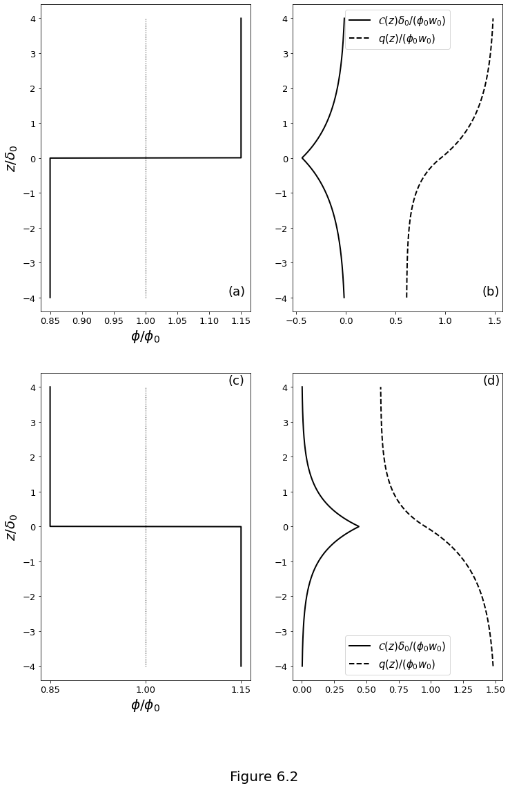
Figure 6.2 plots the porosity, compaction rate, and segregation flux for the permeability-step problem. (a) A porosity increase with \(z\): \(f_m=0.75\), \(f_p=1.25\). (b) Scaled compaction rate and segregation flux for the porosity increase. (c) A porosity decrease with \(z\): \(f_m=1.25\), \(f_p=0.75\). (d) Scaled compaction rate and segregation flux for the porosity decrease.
fig, ax = plt.subplots(2, 2)
fig.set_size_inches(12., 18.)
# Figure 6.2a
fm, fp = 0.85, 1.15
z = np.linspace(-4., 4., 1000)
f = np.asarray([fm if z_ < 0.0 else fp for z_ in z])
ax[0, 0].plot(f, z, '-k', linewidth=2)
ax[0, 0].plot(np.ones(1000), z, ':k', linewidth=1)
ax[0, 0].set_ylabel(r'$z/\delta_0$', fontsize=20)
ax[0, 0].set_xlabel(r'$\phi/\phi_0$', fontsize=20)
ax[0, 0].tick_params(axis='both', which='major', labelsize=13)
ax[0, 0].text(
1.13, -4., '(a)', fontsize=18,
verticalalignment='bottom', horizontalalignment='left'
)
# Figure 6.2b
zmax = 4
n = 3
f0 = 0.01
z = np.linspace(-4., 4., 1000)
C = cmprate(fp, fm, f0, n, z)
fwmW = segflux(fp, fm, f0, n, z)
ax[0, 1].plot(
C, z, '-k', linewidth=2, label='$\mathcal{C}(z)\delta_0/(\phi_0w_0)$'
)
ax[0, 1].plot(fwmW, z,'--k', linewidth=2, label='$q(z)/(\phi_0w_0)$')
ax[0, 1].legend(fontsize=15, loc='upper center')
ax[0, 1].tick_params(axis='both', which='major', labelsize=13)
ax[0, 1].text(
1.37, -4., '(b)', fontsize=18,
verticalalignment='bottom', horizontalalignment='left'
)
# Figure 6.2c
fm, fp = 1.15, 0.85
f = np.asarray([fm if z_ < 0.0 else fp for z_ in z])
ax[1, 0].plot(f, z, '-k', linewidth=2)
ax[1, 0].plot(np.ones(1000), z, ':k', linewidth=1)
ax[1, 0].set_xticks((0.85, 1.0, 1.15))
ax[1, 0].set_ylabel(r'$z/\delta_0$', fontsize=20)
ax[1, 0].set_xlabel(r'$\phi/\phi_0$', fontsize=20)
ax[1, 0].tick_params(axis='both', which='major', labelsize=13)
ax[1, 0].text(
1.13, 4., '(c)', fontsize=18,
verticalalignment='bottom', horizontalalignment='left'
)
# Figure 6.2d
zmax = 4
n = 3
f0 = 0.01
z = np.linspace(-4., 4., 1000)
C = cmprate(fp, fm, f0, n, z)
fwmW = segflux(fp, fm, f0, n, z)
ax[1, 1].plot(C, z, '-k', linewidth=2, label='$\mathcal{C}(z)\delta_0/(\phi_0w_0)$')
ax[1, 1].plot(fwmW, z,'--k', linewidth=2, label='$q(z)/(\phi_0w_0)$')
ax[1, 1].tick_params(axis='both', which='major', labelsize=13)
ax[1, 1].legend(fontsize=15, loc='lower center')
ax[1, 1].text(
1.4, 4., '(d)', fontsize=18,
verticalalignment='bottom', horizontalalignment='left'
)
fig.supxlabel("Figure 6.2", fontsize=20)
plt.show()
Propagation of small porosity disturbances
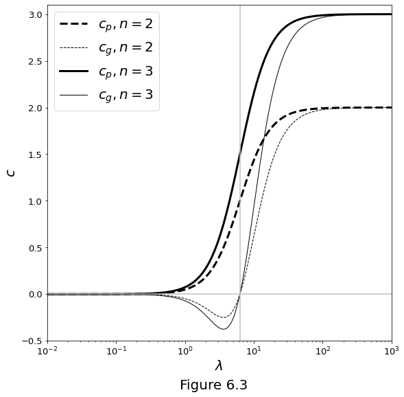
The phase (\(c_p\)) and group (\(c_g\)) velocities are given as
The phase (\(c_p\)) and group (\(c_g\)) velocities are plotted in Figure 6.3 below as a function of the wavelength \(\lambda=2\pi/k\).
lambdas = np.logspace(-2., 3., 1000)
k = 2 * np.pi / lambdas
n = 2.
cp_2 = n/(k ** 2 + 1)
cg_2 = cp_2 - 2. * n * (k**2) / ((k**2 + 1.0) ** 2)
n = 3.
cp_3 = n/(k**2 + 1)
cg_3 = cp_3 - 2. * n * (k**2) / ((k**2 + 1.) ** 2)
fig, ax = plt.subplots()
fig.set_size_inches(9., 9.)
ax.semilogx(lambdas, cp_2, '--k', linewidth=3, label='$c_p, n=2$')
ax.semilogx(lambdas, cg_2, '--k', linewidth=1, label='$c_g, n=2$')
ax.semilogx(lambdas, cp_3, '-k', linewidth=3, label='$c_p, n=3$')
ax.semilogx(lambdas, cg_3, '-k', linewidth=1, label='$c_g, n=3$')
ax.plot([10**(-5), 10**5], [0., 0.], '-', color=[0.75, 0.75, 0.75])
ax.plot([2. * np.pi, 2. * np.pi],[-10., 10.],'-', color=[0.75, 0.75, 0.75])
ax.set_xlabel(r'$\lambda$', fontsize=20)
ax.set_ylabel(r'$c$', fontsize=20)
ax.set_ylim(-0.5, 3.1)
ax.set_xlim(10**(-2), 10**3)
ax.tick_params(axis='both', which='major', labelsize=13)
fig.supxlabel("Figure 6.3", fontsize=20)
plt.legend(fontsize=20)
plt.show()
Magmatic solitary waves
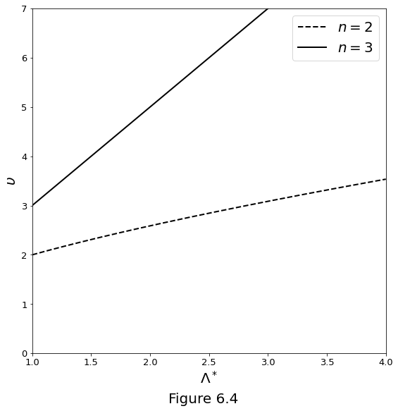
The solitary wave speed \(v\) is computed as
The dimensionless solitary wave speed \(\upsilon\) computed with the equation above as a function of wave amplitude \(\Lambda^*\) relative to the background porosity is plotted in Figure 6.4 below.
fig, ax = plt.subplots()
fig.set_size_inches(9., 9.)
lambdas = np.linspace(1.001, 4., 1000)
c2 = (lambdas - 1.0)**2 / (lambdas * np.log(lambdas) - lambdas + 1.)
c3 = 2. * lambdas + 1.
ax.plot(lambdas, c2, '--k', linewidth=2, label='$n=2$')
ax.plot(lambdas, c3, '-k', linewidth=2, label='$n=3$')
ax.set_xlim(1., 4.)
ax.set_ylim(0., 7.)
ax.set_xlabel(r'$\Lambda^*$', fontsize=20)
ax.set_ylabel(r'$\upsilon$', fontsize=20)
ax.tick_params(axis='both', which='major', labelsize=13)
ax.legend(fontsize=20)
fig.supxlabel("Figure 6.4", fontsize=20)
plt.show()
The normalized porosity profile is obtained through numerical inversion of
which is implemented in Python as
def porosity(f, z, A):
sqrtAf = np.sqrt(A - f)
sqrtAm1 = np.sqrt(A - 1.)
return z + np.sqrt(A + 0.5) * (
-2. * sqrtAf +
np.log(
(sqrtAm1 - sqrtAf)/(sqrtAm1 + sqrtAf)
) / sqrtAm1
)
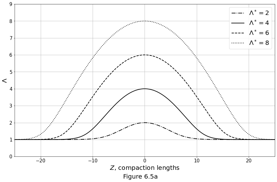
Profiles of normalised porosity perturbation for solitary waves of various amplitude are plotted in Figures 6.5a below. We set \(n=3\) in all cases.
fig, ax = plt.subplots()
fig.set_size_inches(15., 9.)
zmax = 25.
zs = np.linspace(0., zmax, 100)
zm = 0.5 * (zs[1:] + zs[:-1])
AsLS = {2.: '-.', 4.: '-', 6.:'--', 8.: ':'}
phi = {}
for A, ls in AsLS.items():
phi[A] = np.asarray(
[brentq(lambda f: porosity(f, z, A), 1.000000001, A) for z in zs]
)
for A, ls in AsLS.items():
ax.plot(
np.concatenate((-zs[::-1], zs), axis=0),
np.concatenate((phi[A][::-1], phi[A]), axis=0),
'k', label='$\Lambda^* = '+str(int(A))+'$',
linestyle=ls, linewidth=2
)
ax.set_xlim(-zmax, zmax)
ax.set_ylim(0., 9.)
ax.grid()
ax.set_xlabel(r'$Z$, compaction lengths', fontsize=20)
ax.set_ylabel(r'$\Lambda$', fontsize=20)
ax.tick_params(axis='both', which='major', labelsize=15)
ax.legend(fontsize=20)
fig.supxlabel("Figure 6.5a", fontsize=20)
plt.show()
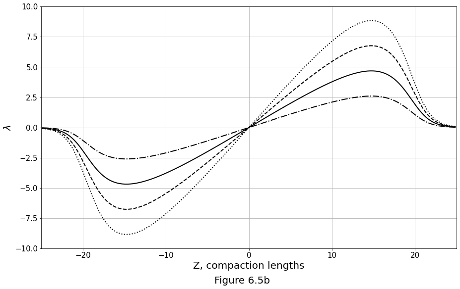
Profiles of compaction rate for solitary waves of various amplitude. \(n=3\) in all cases. The gravity vector \(\gravity\) points to the left, as indicated in the Figure 6.5b below.
fig, ax = plt.subplots()
fig.set_size_inches(15., 9.)
zmax = 25.0
zs = np.linspace(0., zmax, 100)
zm = 0.5 * (zs[1:] + zs[:-1])
AsLS = {2: '-.', 4: '-', 6:'--', 8: ':'}
C = {}
for A, ls in AsLS.items():
# phi is defined in the previous cell
C[A] = -(2. * A + 1.) * (phi[8][1:] - phi[8][0:-1]) / (zs[1] - zs[0])
for A, ls in AsLS.items():
plt.plot(
np.concatenate((-zm[::-1], zm), axis=0),
np.concatenate((-C[A][::-1], C[A]), axis=0),
'k', linestyle=ls, linewidth=2
)
ax.set_xlim(-zmax, zmax)
ax.set_ylim(-10., 10.)
ax.grid()
ax.set_xlabel(r'Z, compaction lengths', fontsize=20)
ax.set_ylabel(r'$\lambda$', fontSize=20)
ax.tick_params(axis='both', which='major', labelsize=15)
fig.supxlabel("Figure 6.5b", fontsize=20)
plt.show()
Solitary-wave trains
The equations below admit a nonlinear solitary wave solution:
which is plotted below:
def get_compaction_rate_dirichlet(phi, n, dz, phi0):
n_ = len(phi)
perm = np.sqrt((phi[:-1] ** n) * (phi[1:] ** n))
# rhs
b = np.zeros(n_, dtype=float)
b[1:-1] = phi0 * dz * (perm[1:] - perm[:-1])
# matrix
offsets = np.array([0, -1, 1])
data = np.zeros(3 * n_).reshape(3, n_)
data[0, 0] = data[0, -1] = 1
data[0, 1:-1] = -(perm[:-1] + perm[1:] + dz * dz) # diagonal
data[1, 0:-2] = perm[:-1] # sub-diagonal
data[2, 2:] = perm[1:] # sup-diagonal
mtx = sps.dia_matrix((data, offsets), shape=(n_, n_))
mtx = mtx.tocsr()
# solution of linear system
Cmp = spla.dsolve.spsolve(mtx, b)
return Cmp
def solitary_wave_update_porosity(PhiOld, n, phi0, dz, dt):
Cmp = get_compaction_rate_dirichlet(PhiOld, n, dz, phi0)
PhiNew = PhiOld + dt * Cmp / phi0
Cmp = 0.5 * (Cmp + get_compaction_rate_dirichlet(PhiNew, n, dz, phi0))
PhiNew = PhiOld + dt * Cmp / phi0
return PhiNew
fig, ax = plt.subplots(figsize=(4.5, 9.0))
ln, = plt.plot([], [], 'k')
phi0 = 0.05 # background porosity
A = 1.5 # amplitude of step
zmax = 150. # total size of domain
z0 = zmax / 5. # location of step
zw = 10. # width of step
n = 3. # permeability exponent
Nz = 1000 # number of grid points
cfl = 1. # courant limit on time-step
tmax = 70. # maximum time
# initial condition
z = np.linspace(0.0, zmax, Nz)
f = 1. - (A - 1.) * (1 + np.tanh((z - z0) / zw)) / 2.
# derived parameters
dz = z[1] - z[0]
V = (1. - phi0 ** n) / (1. - phi0)
dt = cfl * dz / V
Nt = int(np.ceil(tmax / dt))
def init():
ax.set_xlim(0.4, 1.5)
ax.set_ylim(0., zmax)
ax.tick_params(axis='both', which='major', labelsize=13)
return ln,
def update(frame):
global f
f = solitary_wave_update_porosity(f, n, phi0, dz, dt)
ln.set_data(f, z)
return ln,
animation.FuncAnimation(
fig, update, frames=np.linspace(0, tmax, Nt), init_func=init, blit=True
)