Chapter 5 - Material properties¶

%matplotlib inline
import matplotlib.pyplot as plt
import numpy as np
import csv

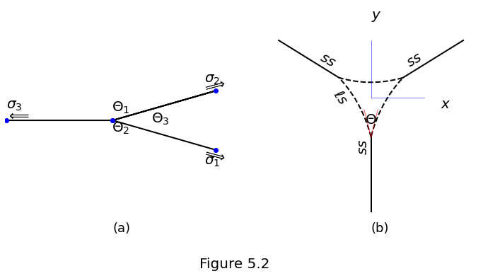
The dihedral angle¶

An equation for dihedral angle $\Theta$ is

$\begin{equation} \label{eq:dihedral-angle} \cos\frac{\dihed}{2} = \frac{\sfce\solsol}{2\sfce\liqsol}. \end{equation}$

Theta = 30.0  # the dihedral angle

Interfaces oriented according to angles $\Theta_k$ and interfacial tensions $\sigma_k$ , as shown in Figure 5.2a.

We can represent the upper liquid–solid interface $y(x)$ as a circular arc-segment with its centre at $(0,y_0)$ and a radius $r_1$ ,

$\begin{split} \begin{align} \label{eq:pore-zero-curvature_y} y(x) &= y_0 \pm \sqrt{r_1^2-x^2},\\ \label{eq:pore-zero-curvature_yp} y'(x) &= \mp\frac{x}{\left({r_1^2-x^2}\right)^{1/2}}, \end{align} \end{split}$

where the sign ( $\pm$ ) is determined by whether the liquid–solid interfaces are concave ( $\Theta<60^\circ$ ) or convex ( $\Theta>60^\circ$ ).

Values for $r_1$ and $y_0$ are obtained by matching the boundary conditions at the pore corners where the interfaces meet at the dihedral angle,

$\begin{split} \begin{align} \label{eq:pore-zero-curvature-bcs-y_J} y(x_\Lambda) &= x_\Lambda\tan(\pi/6)\equiv y_\Lambda,\\ \label{eq:pore-zero-curvature-bcs-y_Jp} y'(x_\Lambda)&=\tan(\pi/6 - \dihed/2)\equiv y'_\Lambda. \end{align} \end{split}$

$x_\Lambda$ is the positive $x$ -position at which the liquid–solid boundary terminates at the solid–solid boundary. Assuming a dihedral angle $\Theta \ne 60^\circ$ and using equations $\eqref{eq:pore-zero-curvature_yp}$ and $\eqref{eq:pore-zero-curvature-bcs-y_Jp}$ we find that

$\begin{equation} \label{eq:circle-pore-radius} r_1 = \frac{x_\Lambda}{y'_\Lambda}\sqrt{1 + {y'_\Lambda}^2}. \end{equation}$

Then, by geometry, $y_0 = y_\Lambda + \text{sgn}(y'_\Lambda)\sqrt{r_1^2 - x_\Lambda^2}$ . These values and equation $\eqref{eq:pore-zero-curvature_y}$ are used to plot the upper interface in Figure 5.2b. The other two interfaces are obtained by rotating the upper interface by $\pm120^\circ$ about the origin.

fig, ax = plt.subplots(1, 2)
fig.set_size_inches(12.0, 6.0)

# Figure 5.2 a

theta_3_rad = Theta * np.pi / 180. / 2.0
thre5_rad = (5. + Theta) * np.pi / 180. / 2.0
thre10_rad = (12. + Theta) * np.pi / 180. / 2.0

factor = lambda t: 0.05 + (0.0 if t > 80. else 0.5*(80. - t)/80.)

ct = np.cos(theta_3_rad)
st = np.sin(theta_3_rad)
x = [-1.0, 0.0, ct, 0.0, ct]
y = [0.0, 0.0, st, 0.0, -st]

ax[0].plot(x, y, '-k', linewidth=2)
ax[0].plot(x, y, 'bo')
ax[0].set_xlim(-1.01, 1.01)
ax[0].set_ylim(-1.01, 1.01)

ax[0].annotate(r'$\Theta_1$', xy=[-0.01, 0.08], fontsize=20)
ax[0].annotate(r'$\Theta_2$', xy=[-0.01, -0.1], fontsize=20)
ax[0].annotate(r'$\Theta_3$', xy=[factor(Theta), -0.02], fontsize=20)

ax[0].text(
    np.cos(thre10_rad), -np.sin(thre10_rad), r'$\sigma_1$', 
    horizontalalignment='center', verticalalignment='center', 
    fontsize=20
)
ax[0].text(
    np.cos(thre5_rad), -np.sin(thre5_rad), r'$\Longrightarrow$', 
    fontsize=20, rotation=-0.5*Theta, 
    horizontalalignment='center', verticalalignment='center'
)
ax[0].text(
    np.cos(thre10_rad), np.sin(thre10_rad), r'$\sigma_2$', fontsize=20, 
    horizontalalignment='center', verticalalignment='center'
)
ax[0].text(
    np.cos(thre5_rad), np.sin(thre5_rad), r'$\Longrightarrow$', 
    fontsize=20, rotation=0.5*Theta, 
    horizontalalignment='center', verticalalignment='center'
)
ax[0].text(
    0.0, -1.0, '(a)', fontsize=18, 
    verticalalignment='bottom', horizontalalignment='left'
)

ax[0].annotate(r'$\sigma_3$', xy=(-1.0, 0.1), fontsize=20, rotation=0.0)
ax[0].annotate(r'$\Longleftarrow$', xy=(-1.0, 0.01), fontsize=20, rotation=0.0)

ax[0].set_axis_off()

# Figure 5.2 b
theta_rad = Theta * np.pi / 180.
beta = 120.*np.pi/180./2.
ysh = 0.2

xI = 0.3 
x = np.linspace(0.0, xI, 100)
y = 0.5 * xI * (
    (x**2/xI**2 - 1.)*np.tan(np.pi/6. - 0.5*theta_rad) 
    + 2.0*np.tan(np.pi/6.)
)
X = np.zeros(x.shape[0] * 2 * 2).reshape(2, 2*x.shape[0])
X[0, :] = np.concatenate((-x[::-1], x), axis=0)
X[1, :] = np.concatenate((y[::-1], y), axis=0)
R = np.array(
    (
        (np.cos(beta*2.), -np.sin(beta*2)), 
        (np.sin(beta*2), np.cos(beta*2))
    )
)
RX = np.fliplr(np.dot(R, X))
RRX = np.fliplr(np.dot(np.linalg.inv(R), X))
x = np.concatenate(
    (np.fliplr(RX)[0, :], X[0,:], np.fliplr(RRX)[0, :]), 
    axis=0
)
y = np.concatenate(
    (np.fliplr(RX)[1, :], X[1,:], np.fliplr(RRX)[1, :]), 
    axis=0
)
ax[1].plot(x, y+ysh, '--k', linewidth=2)

cT = np.cos(beta) 
sT = np.sin(beta)
ss = np.array(((0.0, 0.0), (-1.0, np.amin(y))))
ax[1].plot(ss[0, :], ss[1, :]+ysh, '-k', linewidth=2)
ss = np.dot(np.linalg.inv(R), ss)
ax[1].plot(ss[0, :], ss[1, :]+ysh, '-k', linewidth=2)
ss = np.dot(np.linalg.inv(R), ss)
ax[1].plot(ss[0, :], ss[1, :]+ysh, '-k', linewidth=2)

ax[1].plot([0, 0.5], [ysh, ysh], '-b', linewidth=0.5)
ax[1].plot([0, 0], [ysh, 0.5+ysh], '-b', linewidth=0.5)
ax[1].annotate(
    r'$x$', xy=(0.65, ysh), fontsize=20, 
    verticalalignment='top', horizontalalignment='left'
)
ax[1].annotate(
    r'$y$', xy=(0.0, 0.65+ysh), fontsize=20, 
    verticalalignment='bottom', horizontalalignment='left'
)

f = 0.25
vx = [-f*np.sin(theta_rad/2), 0.0, f*np.sin(theta_rad/2)]
vy = [
    f*np.cos(theta_rad/2) + np.amin(y) +ysh, np.amin(y) + ysh, 
    f*np.cos(theta_rad/2) + np.amin(y) + ysh
]
ax[1].plot(vx, vy, '-r', linewidth=0.6)
ax[1].annotate(
    r'$\Theta$', xy=[0.001, np.amin(y)+ysh+0.09], fontsize=20,
    verticalalignment='bottom', horizontalalignment='center'
)

ax[1].annotate(
    r'$\ell s$', xy=(-0.2, ysh), fontsize=20, rotation=-55., 
    verticalalignment='center', horizontalalignment='right'
)
ax[1].annotate(
    r'$ss$', xy=(0.5, 0.33+ysh), fontsize=20, rotation=30., 
    verticalalignment='center', horizontalalignment='right'
)
ax[1].annotate(
    r'$ss$', xy=(-0.5, 0.33+ysh), fontsize=20, rotation=-30., 
    verticalalignment='center', horizontalalignment='left'
)
ax[1].annotate(
    r'$ss$', xy=(-0.01, -0.5+ysh), fontsize=20, rotation=90., 
    verticalalignment='bottom', horizontalalignment='right'
)

ax[1].text(
    0.0, -1.0, '(b)', fontsize=18, 
    verticalalignment='bottom', horizontalalignment='left'
)

ax[1].set_xlim(-1.01, 1.01)
ax[1].set_ylim(-1.01, 1.01)
ax[1].set_axis_off()

fig.supxlabel("Figure 5.2", fontsize=20)

plt.show()

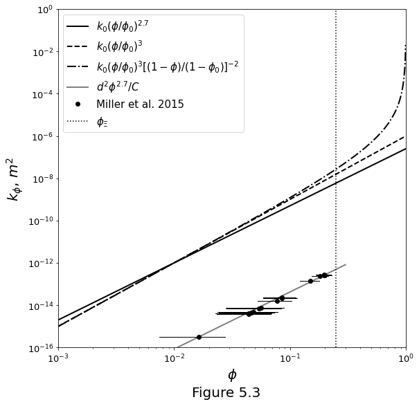
Permeability¶

A simple model which represents the permeability at some reference value of porosity $\phi_0$ is

$\begin{equation} \label{eq:permeability-simple} \perm = k_0(\por/\por_0)^\permexp. \end{equation}$

Equation $\eqref{eq:permeability-simple}$ is plotted in Figure 5.3 below for two values of n. Also shown are permeabilities computed on the basis of simulation of ow through pores of a measured pore geometry.

phi = np.logspace(-3.0, 0.0, 1000, endpoint=False)

phid = 0.25
phi0 = 0.01
K0 = 1e-12

f = phi/phi0

K2 = K0 * (f ** 2.7)
K3 = K0 * (f ** 3.0)
Kkc = K0 * (f ** 3.0) / ((1. - phi)/(1. - phi0)) ** 2

# data and data fit
grainsize = 35e-6
C = 58
permexp = 2.7
dmphi = np.asarray([0.01, 0.3])
dmk = grainsize ** 2 / C * (dmphi ** 2.7)

with open('Data_Permeability_Miller2015.csv', mode='r') as csv_file:
    data = csv.reader(csv_file)
    lst = [row for row in data]
data = np.asarray([[float(l) for l in l_] for l_ in lst[1:]])

fig, ax = plt.subplots()
fig.set_size_inches(9.0, 9.0)

ax.loglog(
    phi, K2, '-k', label=r'$k_0(\phi/\phi_0)^{2.7}$', linewidth=2
)
ax.loglog(
    phi, K3, '--k', label=r'$k_0(\phi/\phi_0)^3$', linewidth=2
)
ax.loglog(
    phi, Kkc, '-.k', linewidth=2,
    label=r'$k_0(\phi/\phi_0)^3[(1-\phi)/(1-\phi_0)]^{-2}$'
)

# data and data fit
ax.loglog(
    dmphi, dmk, '-', color=[0.5, 0.5, 0.5], 
    linewidth=2, label=r'$d^2\phi^{2.7}/C$'
)

ax.loglog(data[:, 0], data[:, -1], 'ok', label=r'Miller et al. 2015')

for d in data:
    ax.plot([d[0]+d[1], d[0]+d[2]], [d[3], d[3]], '-k', linewidth=1)

ax.plot([phid, phid], [1e-16, 1.0], ':k', label=r'$\phi_\Xi$')

ax.set_xlim(1e-3, 1.0)
ax.set_ylim(1e-16, 1.0)
ax.tick_params(axis='both', which='major', labelsize=13)
ax.set_xlabel(r'$\phi$', fontsize=20)
ax.set_ylabel(r'$k_\phi$, $m^2$', fontsize=20)
ax.legend(loc='upper left', fontsize=15)

fig.supxlabel("Figure 5.3", fontsize=20)

plt.show()

The Dynamics of Partially Molten Rock

Chapter 5 - Material properties¶

The dihedral angle¶

Permeability¶