Chapter 12 - Reactive flow and the emergence of melt channels
%matplotlib inline
import matplotlib.pyplot as plt
from matplotlib import gridspec
import numpy as np
from scipy.optimize import fsolve
from scipy.linalg import det, lstsq
from cycler import cycler

import warnings
warnings.filterwarnings('ignore')
Linearised stability analysis
The base state
The assembled, base-state solution is given by
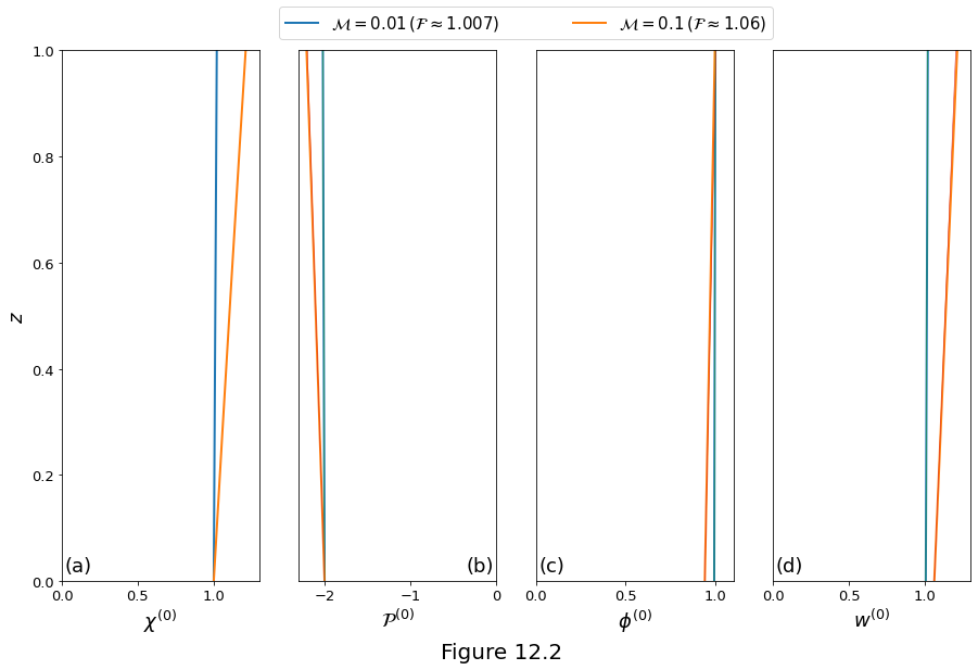
The base-state solutions \(\eqref{eq:rxflow-base-state-solution_1}\)-\(\eqref{eq:rxflow-base-state-solution_4}\) are plotted in Figure 12.2 below for two values of \(\rpro\). Thick lines are the full solution and narrow lines are the linear approximation. In each case, \(\stiff=1\), \(\dpro=1\) and \(\permexp=3\). The values of \(\por\zeroth\) (panel (c)) and \(w\zeroth\) (panel (d)) at \(z=0\) are given by \(\cbasestate^{-1}\) and \(\cbasestate\), respectively.
n = 3.0
G = 1.0
M = np.asarray([0.01, 0.1])
S = 1.0
H = 1.0
z = np.linspace(0.0, H, 1000)

F = np.power([1.0 + S*m*(1+G) for m in M], 1/n)
chi = np.asarray([(1.+G)*np.exp(m*z) - G for m in M])
cmp = -(chi + G)
phi = np.power(
    [chij/(1.0 - S*m*cmpj) for chij, m, cmpj in zip(chi, M, cmp)],
    1.0/n
)
w = chi/phi
cmpl = -(1.0+G) * np.asarray([1.0 + m*z for m in M])
chil = 1.0 + np.asarray([m*(1+G)*z for m in M])
phil = np.asarray(
    [1.0/Fj * (1.0 + m*(1.0 + G)/n*z) for Fj, m in zip(F, M)]
)
wl = np.asarray(
    [Fj*(1.0 + m*(1.0+G)*(1.0-1.0/n)*z) for Fj, m in zip(F, M)]
)
f, ax = plt.subplots(1, 4)
f.set_size_inches(15., 9.)

plt.rc(
    'axes',
    prop_cycle=(
        cycler(color=['k', 'k', 'k', 'k'])
        + cycler(linestyle=['-', '--', ':', '-.'])
    )
)

lines = ax[0].plot(chi.transpose(), z, linewidth=2.0)
ax[0].set_xlabel(r'$\chi^{(0)}$', fontsize=18)
ax[0].set_xlim(0.0, 1.3)
ax[0].set_xticks((0.0, 0.5, 1.0))
ax[0].set_ylabel('$z$', fontsize=18)
ax[0].set_ylim(0.0, 1.0)
ax[0].tick_params(axis='both', which='major', labelsize=13)
ax[0].text(
    0.02, 0.01, '(a)', fontsize=18,
    verticalalignment='bottom', horizontalalignment='left'
)
plt.legend(
    handles=(lines[0], lines[1]),
    labels=(
        r'$\mathcal{M}=0.01\,(\mathcal{F}\approx1.007)$',
        r'$\mathcal{M}=0.1\,(\mathcal{F}\approx1.06)$'
    ),
    fontsize=15, bbox_to_anchor=(-2.5, 1.02, 2.5, .2),
    loc='lower right', ncol=2, mode="expand", borderaxespad=0.
)

ax[1].plot(cmp.transpose(), z, linewidth=2.0)
ax[1].plot(cmpl.transpose(), z, linewidth=0.5)
ax[1].set_xlabel(r'$\mathcal{P}^{(0)}$', fontsize=18)
ax[1].set_xlim(-2.3, 0.0)
ax[1].set_xticks((-2.0, -1.0, 0.0))
ax[1].set_yticks(())
ax[1].set_ylim(0.0, 1.0)
ax[1].tick_params(axis='both', which='major', labelsize=13)
ax[1].text(
    -0.35, 0.01, '(b)', fontsize=18,
    verticalalignment='bottom', horizontalalignment='left'
)

ax[2].plot(phi.transpose(), z, linewidth=2)
ax[2].plot(phil.transpose(), z, linewidth=0.5)
ax[2].set_yticks(())
ax[2].set_xlabel(r'$\phi^{(0)}$', fontsize=18)
ax[2].set_xlim(0.0, 1.1)
ax[2].set_xticks((0.0, 0.5, 1.0))
ax[2].set_ylim(0.0, 1.0)
ax[2].tick_params(axis='both', which='major', labelsize=13)
ax[2].text(
    0.02, 0.01, '(c)', fontsize=18,
    verticalalignment='bottom', horizontalalignment='left'
)

ax[3].plot(w.transpose(), z, linewidth=2)
ax[3].plot(wl.transpose(), z, linewidth=0.5)
ax[3].set_xlabel(r'$w^{(0)}$', fontsize=18)
ax[3].set_yticks(())
ax[3].set_xlim(0.0, 1.3)
ax[3].set_ylim(0.0, 1.0)
ax[3].set_xticks((0.0, 0.5, 1.0))
ax[3].tick_params(axis='both', which='major', labelsize=13)
ax[3].text(
    0.02, 0.01, '(d)', fontsize=18,
    verticalalignment='bottom', horizontalalignment='left'
)

f.supxlabel("Figure 12.2", fontsize=20)

plt.show()
The growth rate of perturbations
The perturbation to the base-state compaction pressure is an ansatz with unknown \(k,m_j,\sigma\), constructed from eigenfunctions of the differential operators, given by
where \(\text{Re}\) means taking only the real part of the complex expression. Equation \(\eqref{eq:rxflow-cbs-ansatz}\) satisfies a linear, partial differential equation that is third order in the \(z\) direction
class PAR:

    def __init__(
        self, F_=1.0, n_=3, S_=1.0, Da_=1000.0, Pe_=100.0, M_=0.01, G_=1,
        bc_=2, nz_=2000, tol_=1e-5, plot_=False, step_=0.01, largeDa_=False
    ):

        self.F = F_         # base - state parameter - force to be constant
        self.n = n_         # permeability exponent
        self.S = S_         # rigidity parameter
        self.Da = Da_       # Damkohler number
        self.Pe = Pe_       # Peclet number
        self.M = M_         # solubility gradient parameter
        self.G = G_         # decompression melting parameter
        self.bc_type = bc_  # boundary condition type -- 1) P(1)=0; 2) P'(1)=0
        self.nz = nz_       # number of points for eigenfunction
        self.tol = tol_     # tolerance
        self.plot = plot_   # plot eigenfunction
        self.step = step_   # stepsize in log10(k) - sigma space
        self.largeDa = largeDa_


class EIG:

    def __init__(self, p_=0.0, phi_=0.0):

        self.P = p_
        self.phi = phi_


class SA:

    def __init__(self, k_=0.0, sigma_=0.0, m_=0.0, flag_=False):

        self.k = k_
        self.sigma = sigma_
        self.m = m_
        self.eig = EIG()
        self.flag = flag_


class DC:

    def __init__(self, s_=0.0, k_=0.0, m_=0.0):

        self.s = s_
        self.k = k_
        self.m = m_
Substituting \(\eqref{eq:rxflow-cbs-ansatz}\) into \(\eqref{eq:rxflow-cbs-por}\) we obtain the characteristic polynomial
where \(\Kk = 1 + k^2/\left(\Da\Pe\right)\). For a given value of \(\sigma\) (which is, in fact, an unknown), equation \(\eqref{eq:characteristic-poly-cbs}\) is solved to obtain the roots \(m_j\).
The function characteristic_polynomial below evaluates the coefficients of the characteristic polynomial.
def characteristic_polynomial(k, sig, par):

    k2 = k[0] * k[0] if type(k) is np.ndarray else k * k
    K_ = k2 / par.Da / par.Pe / par.F + 1.0
    # cubic
    p3 = 0.0 if par.largeDa else sig / par.Da
    # quadratic
    p2 = sig * K_ - par.n * np.power(
        par.F, 1 + par.n
    ) / par.Da / par.S
    # linear
    p1 = -(
        par.n * np.power(
            par.F, 1 + par.n
        ) * K_ / par.S + sig * k2 / par.Da
    )
    # constant
    p0 = k2 * (par.n * np.power(par.F, 1 - par.n) - sig * K_)
    p = np.array([p3, p2, p1, p0])

    return p.reshape(p.shape[0])
The boundary conditions impose zero perturbation of the base-state along the bottom boundary. Hence we take \(\usat\first=\por\first=w\first=0\) at \(z=0\). Moreover, we require that perturbations to the flow are unimpeded (and unforced) by gradients in the compaction pressure at the top of the domain, \(z=1\). Using these boundary conditions and equations \(\eqref{eq:rxflow-base-state-solution_1}\)-\(\eqref{eq:rxflow-base-state-solution_4}\) we find that
This set of conditions must hold for all \(x\) and \(t>0\). Combining these conditions with our ansatz \(\eqref{eq:rxflow-cbs-ansatz}\) and expressing in terms of a matrix-vector multiplication gives
The Python function boundary_condition_matrix implements the system of equations \(\eqref{eq:rxflow_cbs_matrix_eqn}\).
def boundary_condition_matrix(k, m, sig, par):

    if par.bc_type == 1:
        M = np.array(
            [[1.0, mi, np.exp(mi)] for mi in m]
        ).transpose()
    elif par.bc_type == 2:
        M = np.array(
            [[1.0, mi, mi * np.exp(mi)] for mi in m]
        ).transpose()
    elif par.bc_type == 3:
        q = sig * par.S / par.n
        M = np.array([[
            q * mi - 1.0,
            q * mi * mi - mi - q * k ** 2,
            mi * np.exp(mi)
        ] for mi in m]).transpose()
    else:
        q = k * k * par.Da / par.DaPe
        M = np.array(
            [[1.0 - par.S * mi,
            mi * mi + q * mi,
            mi * np.exp(mi)]
            for mi in m]
        ).transpose()

    return M
def zero_by_sigma_or_wavenumber(sig, k, par):

    m = np.roots(characteristic_polynomial(k, sig, par))

    if par.largeDa:
        residual = np.real(m[0]) * np.sin(np.imag(m[0])) + \
            np.imag(m[0]) * np.cos(np.imag(m[0]))
    else:
        detM = det(boundary_condition_matrix(k, m, sig, par))
        residual = np.real((1. - 1.j) * detM)

    return residual
def form_eigenfunction(k, sigma, par):

    m = np.roots(characteristic_polynomial(k, sigma, par))
    z = np.linspace(0.0, 1.0, par.nz)
    eig = EIG()

    if par.largeDa:
        eig.P = np.exp(np.real(m[0]) * z) * np.sin(np.imag(m[0]) * z)
        eig.P = eig.P / np.max(np.abs(eig.P))
        Q = (m[0] ** 2 - k ** 2) * eig.P
        eig.phi = np.power(par.F, -1.0 - par.n) * \
            par.S / par.n * np.cumsum(Q) * (z[1] - z[0])
    else:
        M = boundary_condition_matrix(k, m, sigma, par)
        subM = M[:, 1:]
        b = -M[:, 0]
        A = (1.+0.j) * np.ones(3)
        A[1:] = lstsq(subM, b)[0]

        eig.P = np.zeros_like(z, dtype=np.complex128)
        Q = np.zeros_like(z, dtype=np.complex128)
        for Aj, mj in zip(A, m):
            tmp = Aj * np.exp(mj * z)
            eig.P += tmp
            Q += (mj * mj - k * k) * tmp

        eig.phi = np.power(par.F, -1 - par.n) * \
            par.S / par.n * np.cumsum(Q) * (z[1] - z[0])

    return eig
Function reactive_flow_solve_dispersion below implements a recipe for obtaining solutions: for a given set of parameters \(\permexp\), \(\stiff\), \(\Da\), \(\Pe\) and a chosen horizontal wavenumber \(k\), form an initial guess of \(\sigma\). Using this guess, obtain the three roots of the characteristic polynomial \(\eqref{eq:characteristic-poly-cbs}\). Use these roots to form the residual \(r\). If \(r\) is below a specified tolerance, accept the guess of \(\sigma\) as a solution; otherwise, improve the guess of \(\sigma\) (using, for example, \(\infd r/\infd\sigma\) and Newton’s method) and again form the residual. Repeat this until the tolerance has been satisfied. Then, with the converged value for \(\sigma\), obtain the roots \(m_j\), take \(A_1=1\), and solve the system of equations \(\eqref{eq:rxflow_cbs_matrix_eqn}\) for \(A_2\) and \(A_3\). Use the values of \(A_j\) to form the eigenfunction \(\cmppres\first\) at \(t=0\).
def reactive_flow_solve_dispersion(k_guess, sigma_guess, par, verbose=False):

    sa = SA()

    if type(k_guess) is not np.ndarray:
        # solving for growthrate sigma at a fixed value of wavenumber k
        solve_for_sigma = True
        sa.k = k_guess
        if sigma_guess is None:
            sigma_guess = np.logspace(-1.0, 1.0, 100)
        if type(sigma_guess) is not np.ndarray:
            sigma_guess = np.asarray([sigma_guess])
    else:
        # solving for wavenumber k at a fixed value of growthrate sigma
        solve_for_sigma = False

        if type(sigma_guess) is not np.ndarray:
            sa.sigma = sigma_guess
        else:
            sa.sigma = sigma_guess[0]

    if par.F is None:
        par.F = np.power(1.0 + par.S * par.M * (1.0 + par.G), 1.0 / par.n)

    sigma = np.zeros_like(sigma_guess)
    k = np.zeros_like(k_guess)

    if solve_for_sigma:
        # solve eigenvalue problem to find growth rate of fastest-growing mode
        res = np.zeros_like(sigma_guess)
        exitflag = np.zeros_like(sigma_guess)
        converged = np.zeros_like(sigma_guess)
        problem_sigma = lambda s: zero_by_sigma_or_wavenumber(s, sa.k, par)

        for j in range(len(sigma_guess)):

            [sigma[j], infodict, exitflag[j], _] = fsolve(
                problem_sigma, sigma_guess[j], full_output=True, xtol=1.e-14
            )
            res[j] = infodict["fvec"]
            converged[j] = exitflag[j] == 1 and np.abs(res[j]) < par.tol

            if par.largeDa:
                m = np.roots(
                    characteristic_polynomial(sa.k, sigma[j], par)
                )
                converged[j] = \
                    converged[j] and np.pi / 2 < np.abs(np.imag(m[0])) < np.pi

            if par.plot and converged[j] == 1:
                eig = form_eigenfunction(sa.k, sigma[j], par)

    else:
        # solve eigenvalue problem to find wavenumber of mode
        problem_wavenumber = lambda s: zero_by_sigma_or_wavenumber(sa.sigma, s, par)
        res = np.zeros_like(k_guess)
        exitflag = np.zeros_like(k_guess)
        converged = np.zeros_like(k_guess)
        for j in range(len(k_guess)):

            [k[j], infodict, exitflag[j], _] = fsolve(
                problem_wavenumber, k_guess[j], full_output=True, xtol=1.e-14
            )
            res[j] = infodict["fvec"]
            converged[j] = exitflag[j] == 1 or abs(res[j]) < par.tol

            if par.largeDa:
                m = np.roots(characteristic_polynomial(k[j], sa.sigma, par))
                converged[j] = \
                    converged[j] and np.pi / 2 < np.abs(np.imag(m[0])) < np.pi

            if par.plot and converged[j] == 1:
                eig = form_eigenfunction(k[j], sa.sigma, par)
                plt.plot(np.linspace(0.0, 1.0, par.nz), np.real(eig.P))

    none_converged = not np.sum(converged)

    # handle failure to find solution
    if none_converged:
        if verbose:
            print(f'FAILURE: no solution found for k={k_guess}')
        sa.sigma = np.nan
        sa.k = np.nan
        sa.m = [np.nan, np.nan, np.nan]
        sa.eig.P = np.nan
        sa.flag = False
        return sa
    elif solve_for_sigma:
        sa.sigma = np.amax(sigma[converged != 0])
    else:
        sa.k = np.amax(k[converged != 0])

    sa.m = np.roots(characteristic_polynomial(sa.k, sa.sigma, par))

    # form and check eigenfunction
    sa.eig = form_eigenfunction(sa.k, sa.sigma, par)
    gP = np.gradient(sa.eig.P)

    if (gP < 0).any() and par.bc_type != 1:
        sa.flag = False
        if verbose:
            print(
                'FAILURE: non-monotonic eigenfunction ' +
                f' for k={sa.k}, sigma={sa.sigma}'
            )
    else:
        sa.flag = True
        if verbose:
            print(
                'SUCCESS: monotonic eigenfunction ' +
                f' for k={sa.k}, sigma={sa.sigma}'
            )

    if par.plot:
        plt.plot(
            np.linspace(0, 1, par.nz), np.real(sa.eig.P), linewidth=2
        )

    return sa
def taylor_series_extension(n, x, y, step, init_Lks):

    if n == 0:
        xguess = init_Lks[0]
        yguess = init_Lks[1]
    elif n == 1:
        xguess = x[0]-step
        yguess = y[0]
    elif n == 2:
        d = np.asarray([x[1]-x[0], y[1]-y[0]])
        d = d/np.sqrt(np.sum(d**2))
        xguess = x[-1] + d[0]*step
        yguess = y[-1] + d[1]*step
    else:
        da = np.asarray([x[-1]-x[-2], y[-1]-y[-2]])
        db = np.asarray([x[-2]-x[-3], y[-2]-y[-3]])
        D = 0.5*(np.sqrt(np.sum(da**2)) + np.sqrt(np.sum(db**2)))
        da = da/np.sqrt(np.sum(da**2))
        db = db/np.sqrt(np.sum(db**2))
        d2 = (da - db)/D
        xguess = x[-1] + da[0]*step + 0.5*d2[0]*step**2
        yguess = y[-1] + da[1]*step + 0.5*d2[1]*step**2

    if np.isinf(xguess) or np.isnan(xguess):
        xguess = x[-1]
    if np.isinf(yguess) or np.isnan(yguess):
        yguess = y[-1]

    return xguess, yguess
def reactive_flow_trace_dispersion_curve(
    par, Lkbounds, sbounds, init_Lks, verbose=False
):

    n = 0  # can n be zero?
    Lk = np.full((1, ), np.inf)  # dictionaries
    s = np.full((1, ), np.inf)
    m = np.full((1, 2), np.inf + 0.j, dtype=complex) if par.largeDa \
        else np.full((1, 3), np.inf + 0.j, dtype=complex)

    for j in [0, 1]:

        fails = 0
        while n < 1_000_000:

            Lk_guess, s_guess = taylor_series_extension(n, Lk, s, par.step, init_Lks)

            if Lk_guess <= Lkbounds[0] or Lk_guess >= Lkbounds[1]:
                break
            if s_guess <= sbounds[0] or s_guess >= sbounds[1]:
                break

            if n == 0:
                s_guess = np.linspace(0.1, par.n, 30)

            elif fails <= 1:
                if verbose and (n % 50 == 0 or n == 0):
                    print(
                        f'Iteration {n}: ' +
                        f' searching for solution at k={np.power(10, Lk_guess)}'
                    )
                s_guess = s_guess * np.linspace(0.99, 1.01, 16)

            elif fails == 2:
                if verbose and (n % 50 == 0 or n == 0):
                    print(
                        f'Iteration {n}: ' +
                        f' searching for solution at sigma={s_guess}'
                    )
                Lk_guess = Lk_guess * np.linspace(0.99, 1.01, 16)

            else:
                break

            sa = reactive_flow_solve_dispersion(
                np.power(10., Lk_guess), s_guess, par
            )

            if sa.flag:
                # found lowest mode; prepare for next iteration
                if n == 0:
                    Lk[n] = np.log10(sa.k)
                    s[n] = sa.sigma
                    m[n] = sa.m
                else:
                    Lk = np.concatenate((Lk, np.asarray([np.log10(sa.k)])))
                    s = np.concatenate((s, np.asarray([sa.sigma])))
                    m = np.concatenate((m, np.asarray([sa.m])))
                n = n + 1
                fails = 0
            else:
                # found higher mode; retry
                fails = fails + 1

        if j == 0:
            s = np.flip(s)
            Lk = np.flip(Lk)
            m = np.flipud(m)

    return DC(s, np.power(10., Lk), m)
par = PAR()

Lkbounds = np.log10([0.1, 400.0])
sbounds = np.asarray([0.05, 4.0])
init_Lks = np.asarray([np.log10(5.0), 3.0])

DC_ref = reactive_flow_trace_dispersion_curve(par, Lkbounds, sbounds, init_Lks)
iref = np.argmax(DC_ref.s)
dpar = PAR()
dpar.Da = 10.0
DC_a = reactive_flow_trace_dispersion_curve(dpar, Lkbounds, sbounds, init_Lks)
dpar = PAR()
dpar.Da = 100.0
DC_b = reactive_flow_trace_dispersion_curve(dpar, Lkbounds, sbounds, init_Lks)
k_iref, s_iref = DC_ref.k[iref], DC_ref.s[iref]
par = PAR()
SA_ref = reactive_flow_solve_dispersion(k_iref, s_iref, par)

lambda_ = 2.0 * np.pi/k_iref
X, Z = np.meshgrid(
    np.linspace(0.0, 2.0 * lambda_, par.nz),
    np.linspace(0.0, 1.0, par.nz)
)
P = np.real(
    np.tile(SA_ref.eig.P, (par.nz, 1)).transpose() * \
        np.exp(1j * k_iref * X)
)
phi = np.real(
    np.tile(SA_ref.eig.phi, (par.nz, 1)).transpose() * \
        np.exp(1j * k_iref * X)
)
epsilon = 3.e-5
h = 0.1/(par.nz+1.0)
hx = X[0,1] - X[0,0]
hz =  Z[1,0] - Z[0,0]
Pz, Px = np.gradient(P, hz, hx)
F = par.F
U = epsilon * np.real(- par.S * Px)
W = F + epsilon * np.real((par.n-1) * phi - par.S * Pz)
Chi = s_iref * phi - P

P = np.real(P)
P = (P - np.amin(P))/(np.amax(P) - np.amin(P))
phi = np.real(phi)
phi = (phi - np.amin(phi))/(np.amax(phi) - np.amin(phi))
Chi = np.real(Chi)
Chi = (Chi - np.amin(Chi))/(np.amax(Chi) - np.amin(Chi))
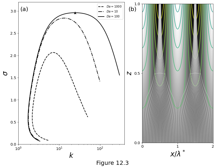
Figure 12.3 below illustrates the results of numerical solutions of the stability problem. (a) Dispersion curves: growth rate \(\sigma\) as a function of wavenumber \(\wavenumber\) from numerical solutions for \(\sigma,m_j,A_j\) for three different values of \(\Da\). All three curves use the parameters \(\Pe=100,\,\rpro=0.01,\,\dpro=\stiff=1\) and \(\permexp=3\) (corresponding to the parameters used to compute the base state in the Figure above). The star symbol marks the maximum growth rate for the reference curve. (b) The eigenmode with maximum growth rate \(\sigma^*\approx 2.96\) at \(\wavenumber^*\approx 24.6\) (\(\lambda^*\approx0.26\)) for the curve with \(\Da=1000\) corresponding to the star marker in panel (a). The perturbation to the compaction pressure \(\cmppres\first\) is shown in the grayscale background image. The narrow lines are contours of the porosity perturbation \(\por\first\), which has maxima where the compaction pressure has minima. The white curves are streamlines of the flow \(\vel\liq = \zhat + \smallpar\vel\first\), with \(\smallpar\) chosen to be \(3\times10^{-5}\). The velocity perturbation \(\vel\first\) is computed with equation \(\vel\first = \left(\permexp - 1\right)\por\first\zhat - \stiff\Grad\cmppres\first\).
f, ax = plt.subplots()
f.set_size_inches(12.0, 9.0)

gs = gridspec.GridSpec(1, 2, width_ratios=[1.5, 1])

ax0 = plt.subplot(gs[0])
ax0.plot(DC_a.k, DC_a.s, '--k', linewidth=2, label=r'$Da=1000$')
ax0.plot(DC_b.k, DC_b.s, '-.k', linewidth=2, label=r'$Da=10$')
ax0.plot(DC_ref.k, DC_ref.s, '-k', linewidth=2, label=r'$Da=100$')
ax0.plot(DC_ref.k[iref], DC_ref.s[iref], '*k', markersize=9)
ax0.set_xlabel(r'$k$', fontsize=24)
ax0.set_xscale('log')
ax0.set_xlim(1.0, 400.0)
ax0.set_xticks((1e0, 1e1, 1e2))
ax0.set_ylim(0.0, 3.2)
ax0.set_ylabel(r'$\sigma$', fontsize=24)
ax0.tick_params(axis='both', which='major', labelsize=13)
ax0.text(
    1.1, 3.1, '(a)', fontsize=20,
    verticalalignment='top', horizontalalignment='left'
)
ax0.legend()

ax1 = plt.subplot(gs[1])
ax1.imshow(np.flipud(P), cmap='gray', extent=[0.0, 2.*lambda_, 0.0, 1.0])
ax1.contour(X, Z, phi, levels=np.linspace(-1, 1, 20))
nlines = 48
h = 2.0 * lambda_/(nlines+1.0)
seed = np.zeros((nlines, 2))
seed[:, 0] = np.linspace(0.5*h, 2.0*lambda_-0.5*h, nlines)
seed[:, 1] = 0.001
ax1.streamplot(
    X, Z, U, W, start_points=seed,
    integration_direction='forward', density=(90, 60),
    color=[0.8, 0.8, 0.8], arrowstyle='-'
)
ax1.set_xlabel(r'$x/\lambda^*$', fontsize=24)
ax1.set_xlim(0, 2.*lambda_)
ax1.set_xticks((0, lambda_, 2*lambda_))
ax1.set_xticklabels((0, 1, 2))
ax1.set_ylabel(r'$z$', fontsize=24)
ax1.set_ylim(0.0, 1.0)
ax1.set_yticks((0, 0.5, 1))
ax1.tick_params(axis='both', which='major', labelsize=13)
ax1.text(
    -0.04, 0.98, '(b)', fontsize=20,
    verticalalignment='top', horizontalalignment='right'
)

f.supxlabel("Figure 12.3", fontsize=20)

plt.show()
The large-Damköhler number limit
Considering the asymptotic limit of large Damköhler number, we can reduce the polynomial \(\eqref{eq:characteristic-poly-cbs}\) to second order,
The function characteristic_polynomial above already includes this case and evaluatees the coefficients of the both characteristic polynomial \(\eqref{eq:characteristic-poly-cbs}\) and \(\eqref{eq:characteristic-poly-quad}\).
Lkbounds = np.log10([0.1, 400.0])
sbounds = np.asarray([0.05, 4.0])
init_Lks = np.asarray([np.log10(5.0), 3.0])
DC_cube = {}
DC_quad = {}

for vals in [10., 100., 1000.]:

    par = PAR(Da_=vals, largeDa_=False)
    DC_cube[vals] = reactive_flow_trace_dispersion_curve(
        par, Lkbounds, sbounds, init_Lks
    )

    par = PAR(Da_=vals, largeDa_=True)
    DC_quad[vals] = reactive_flow_trace_dispersion_curve(
        par, Lkbounds, sbounds, init_Lks
    )
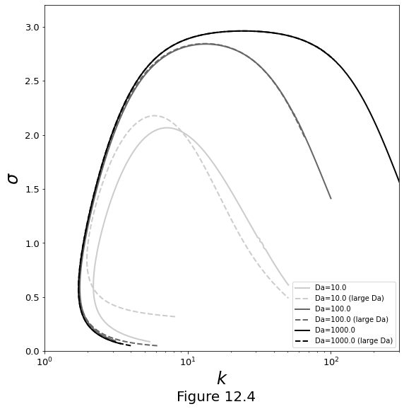
Figure 12.4 below plots the dispersion curves for growth rate \(\sigma\) as a function of wavenumber \(\wavenumber\). Curves come from numerical solutions to the full problem (cubic polynomial \(\eqref{eq:characteristic-poly-cbs}\), solid lines) and the large-\(\Da\) problem (quadratic \(\eqref{eq:characteristic-poly-quad}\), dashed lines). The agreement for \(\Da \ge 100\) suggests that the large-Damköhler approximation is very good for geologically relevant conditions.
f, ax = plt.subplots()
f.set_size_inches(9., 9.)

for vals, gray in zip([10., 100., 1000.], [0.8, 0.4, 0.]):

    plt.plot(
        DC_cube[vals].k, DC_cube[vals].s, '-', linewidth=2,
        color=[gray, gray, gray], label=r'Da='+str(vals)
    )
    plt.plot(
        DC_quad[vals].k, DC_quad[vals].s, '--', linewidth=2,
        color=[gray, gray, gray], label=r'Da=' + str(vals) + ' (large Da)'
    )

plt.xscale('log')
plt.xlim(1, 300)
plt.xlabel(r'$k$', fontsize=24)
plt.ylim(0, 3.2)
plt.ylabel(r'$\sigma$', fontsize=24)
plt.legend()
plt.tick_params(axis='both', which='major', labelsize=13)
f.supxlabel("Figure 12.4", fontsize=20)
plt.show()
A modified problem and its analytical solution
It is possible to obtain an algebraic equation that can be solved for the growth-rate \(\sigma\) as a function of wavenumber \(k\) and parameters \(\permexp,\Da,\Pe,\stiff\) (recall that \(\Kk = 1 + k^2/(\Da\Pe)\)). Without any approximations, the growth rate of \(l=1\) perturbations is given by
The function ReactiveFlowAnalyticalSolution below takes \(k, \permexp,\Da,\Pe,\stiff\) as arguments and evaluates the value of \(\sigma\) given by equation \(\eqref{eq:rxflow-analytical-sigma-full}\).
class PAR_MOD:
    def __init__(self):
        self.s = None
        self.k = None
        self.smax = None
        self.kmax = None
        self.X = None
        self.Y = None
        self.P = None
        self.phi = None
        self.U = None
        self.W = None


def ReactiveFlowAnalyticalSolution(k, n, Da, Pe, S):
    K = (1 + k*k / Da / Pe).astype(np.clongdouble)
    b = np.pi
    # growth rate - upper branch
    full = np.zeros((k.shape[0], 2), dtype=np.clongdouble)
    b2 = b ** 2
    Da2 = Da ** 2
    Da3 = Da ** 3
    Da4 = Da ** 4
    K2 = K ** 2
    K4 = K ** 4
    k2 = k ** 2
    k4 = k ** 4
    k6 = k ** 6
    S2 = S ** 2
    full[:, 0] = (
        2.0 * n * np.sqrt(
            -Da4 * K4 * b2 - Da4 * K4 * k2 + Da4 * K2 * S2 * k4
            - 3.0 * Da3 * K2 * S * k4 - 2 * Da2 * K2 * b2 * k2
            - Da * S * k6 - b2 * k4
        )
        + 4 * Da * K * b2 * n + Da * K * k2 * n
        + 2 * Da2 * K * S * k2 * n
    ) / (
        4 * S * Da2 * K2 * b2 + 4 * S * Da2 * K2 * k2 + S * k4
    )
    # lower branch
    full[:, 1] = -(
        2.0 * n * np.sqrt(
            - Da4 * K4 * b2 - Da4 * K4 * k2
            + Da4 * K2 * S2 * k4 - 3 * Da3 * K2 * S * k4
            - 2 * Da2 * K2 * b2 * k2 - Da * S * k6 - b2 * k4
        )
        - K * (4 * Da * n * b2 + n * (2 * S * Da2 + Da) * k2)
    ) / (
        S * (4 * Da2 * K2 * b2 + 4 * Da2 * K2 * k2 + k4)
    )

    real1 = np.nonzero(
        np.imag(full[:, 0]).astype(np.float32) == 0.0
    )
    real2 = np.nonzero(
        np.imag(full[:, 1]).astype(np.float32) == 0.0
    )
    s = PAR_MOD()
    s.s = np.real(
        np.concatenate((
            np.flipud(full[real1, 0].flatten()),
            full[real2, 1].flatten()
        ))
    )
    s.k = np.real(
        np.concatenate((
            np.flipud(k[real1].flatten()), k[real2].flatten()
        ))
    )
    I = np.argmax(s.s)
    s.smax = s.s[I]
    s.kmax = s.k[I]

    # eigenfunctions
    K = 1 + s.kmax ** 2 / Da / Pe
    a = 0.5 * (
        n * K / S + s.smax * s.kmax ** 2 / Da
    ) / (
        s.smax * K - n / Da / S
    )
    m = a + 1j * np.pi
    lambda_ = 2 * np.pi / s.kmax
    x = np.linspace(0, 2 * lambda_, 1000)
    hx = x[2]-x[1]
    y = np.linspace(0, 1, 1000)
    hy = y[2]-y[1]
    s.X, s.Y = np.meshgrid(x, y)
    s.P = np.exp(a * s.Y) * np.sin(np.pi * s.Y) * np.sin(s.kmax * s.X)
    tmp = np.exp(a * s.Y) * np.cos(np.pi * s.Y) * np.sin(s.kmax * s.X)
    dphi_dy = S * (
        (a ** 2 - np.pi ** 2 - s.kmax ** 2) * s.P + 2 * a * np.pi * tmp
    ) / n
    s.phi = np.cumsum(dphi_dy, axis=0) * hy

    Py, Px = np.gradient(s.P, hy, hx)
    s.U = -S * Px
    s.W = (n - 1) * s.phi - S * Py

    s.P = (s.P - np.amin(s.P)) / (np.amax(s.P) - np.amin(s.P))
    s.phi = (s.phi - np.amin(s.phi)) / (np.amax(s.phi) - np.amin(s.phi))

    return s
n = 3.
Da = 1000.
Pe = 100.
S = np.asarray([0.01, 0.1, 1, 10]).astype(np.clongdouble)
k = np.logspace(-1.0, 4.0, 10000).astype(np.clongdouble)
s = []

for s_ in S:

    s.append(ReactiveFlowAnalyticalSolution(k, n, Da, Pe, s_))
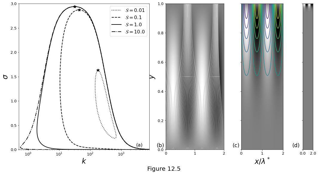
Figure 12.5 below plot the results for the modified problem with \(\cmppres\first=0\) at \(z=1\). (a) Dispersion curves for \(n=3\), \(\Da=1000\), \(\Pe=100\) and four values of \(\stiff\). Maximum values of the growth rate for each curve are marked by stars. The eigenfunctions for each of these maxima are plotted in subsequent panels. (b) The \(\cmppres\first\) eigenfunction for \(\stiff=1\). White curves are streamlines of the flow \(\vel\liq = \zhat + \smallpar\vel\first\), with \(\smallpar\) chosen to be \(3\times10^{-3}\). (c) \(\cmppres\first\) for \(\stiff=0.1\) with superimposed contours of the porosity perturbation \(\por\first\). Porosity is larger in the low-pressure channels. (d) \(\cmppres\first\) for \(\stiff=0.01\).
fig = plt.figure(figsize=(18., 9.))
gs = gridspec.GridSpec(1, 4, width_ratios=[6, 3, 2, 1])

ax0 = plt.subplot(gs[0])

for s_, lstyi, S_ in zip(s, {'--k', '-k', '-.k', ':k'}, S):
    ax0.semilogx(
        s_.k, s_.s, lstyi, linewidth=2,
        label=r'$\mathcal{S}=' + str(np.real(S_).astype(np.float32)) + '$'
    )
    ax0.plot(
        s_.kmax, s_.smax, '*k', linewidth=1, markersize=10
    )

ax0.set_xlabel(r'$k$', fontsize=24)
ax0.set_xlim(0.5, 8000)
ax0.set_xticks(ticks=(1.e0, 1.e1, 1.e2, 1.e3))
ax0.set_ylabel(r'$\sigma$', fontsize=24)
ax0.set_ylim(0.0, 3.0)
ax0.legend(fontsize=16)
ax0.tick_params(axis='both', which='major', labelsize=13)
ax0.text(
    0.5e4, 0.05, '(a)', fontsize=16,
    verticalalignment='bottom', horizontalalignment='right'
)

AR = 2 * np.pi / np.asarray([s[2].kmax, s[1].kmax, s[0].kmax])

ax1 = plt.subplot(gs[1])
lambda_ = np.float32(AR[0])
ax1 = plt.subplot(gs[1])
ax1.imshow(
    np.real(s[2].P).astype(np.float32), cmap='gray',
    extent=[0.0, 2.*lambda_, 0.0, 1.0]
)
ax1.set_ylabel(r'$y$', fontsize=24)
nlines = 48
h = 2 * lambda_ / (nlines + 1)
seed = np.zeros((nlines, 2))
seed[:, 0] = np.linspace(0.5 * h, 2.0 * lambda_ - 0.5 * h, nlines)
seed[:, 1] = 0.001
epsilon = 3e-3
U = epsilon * np.real(s[2].U).astype(np.float64)
W = 1. + epsilon * np.real(s[2].W).astype(np.float64)
x = np.linspace(0., 2. * lambda_, 1000)
y = np.linspace(0., 1., 1000)
X, Y = np.meshgrid(x, y)

ax1.streamplot(
    X, Y, U, W, start_points=seed,
    integration_direction='forward', density=(90, 60),
    color=[0.8, 0.8, 0.8], arrowstyle='-'
)

ax1.set_xticks((0, AR[0], 2*AR[0]))
ax1.set_xticklabels((0, 1, 2))
ax1.tick_params(axis='both', which='major', labelsize=13)
ax1.text(
    -0.01, 0.01, '(b)', fontsize=18,
    verticalalignment='bottom', horizontalalignment='right'
)

ax2 = plt.subplot(gs[2])
lambda_ = np.float32(AR[1])
ax2 = plt.subplot(gs[2])
ax2.imshow(
    np.flipud(np.real(s[1].P)).astype(np.float32), cmap='gray',
    extent=[0.0, 2.*lambda_, 0.0, 1.0]
)
x = np.linspace(0, 2 * lambda_, 1000)
y = np.linspace(0, 1, 1000)
X, Y = np.meshgrid(x, y)
ax2.contour(
    X, Y, np.real(s[1].phi).astype(np.float32),
    levels=np.linspace(0, 1, 12)
)
ax2.set_xticks((0, lambda_, 2*lambda_))
ax2.set_xticklabels((0, 1, 2))
ax2.set_yticklabels(())
ax2.set_xlabel(r'$x/\lambda^*$', fontsize=24)
ax2.tick_params(axis='both', which='major', labelsize=13)
ax2.text(
    -0.01, 0.01, r'(c)', fontsize=18,
    verticalalignment='bottom', horizontalalignment='right'
)

ax3 = plt.subplot(gs[3])
lambda_ = np.float32(AR[2])
ax3.imshow(
    np.flipud(np.real(s[0].P)).astype(np.float32),
    cmap='gray', extent=[0.0, 2.*lambda_, 0.0, 1.0]
)
ax3.set_xticks((0, 2*lambda_))
ax3.set_xticklabels((0., 2.))
ax3.set_yticklabels(())
plt.text(
    -0.02, 0.01, r'(d)', fontsize=18,
    verticalalignment='bottom', horizontalalignment='right'
)
ax3.tick_params(axis='both', which='major', labelsize=13)

fig.supxlabel("Figure 12.5", fontsize=20)

plt.show()
Equation \(\eqref{eq:rxflow-analytical-sigma-full}\) is exact but difficult to analyse. We therefore design an approximation to be valid only near the peak growth rate:
and substitute, dropping the \(\permexp/\Da\stiff\) terms. We find that
Here we have made the additional approximation that near the maximum growth rate (i.e., for \(\wavenumber\approx\wavenumber^*\) at which \(\epsilon \ll 1\)), \(\wavenumber^2/\Da\Pe \ll 1\) and hence that \(\Kk \sim 1\).
The maximum growth rate \(\sigma\sim\sigma^*\) occurs where \(\epsilon\) is at a minimum with respect to \(\wavenumber\). Using equations \(\eqref{eq:rxflow-analytic-real-im-asymptotic_a}\) - \(\eqref{eq:rxflow-analytic-real-im-asymptotic_e}\) we find that
where \(\mathcal{B} \equiv b^2 + (2\stiff)^{-2}\). The maximum growth rate \(\sigma^*\) of the channel instability is
class SA_Growth():

    def __init__(self):

        self.k = None
        self.a = None
        self.e = None
        self.s = None


def asym_maxgrowth(k, n, Da, Pe, S, l):

    b = l * np.pi
    B = b**2 + 1.0/4.0/S**2
    s_ = SA_Growth()
    k = np.power(4.0*Da*Pe*(b**2 + 1.0/4.0/S**2)/(4.0 + Pe/Da), 0.25)
    a = 1.0/2.0/S + k**2.0/2.0/Da
    e = (a**2 + b**2)/k**2 + k**2/Da/Pe
    s = n * (1.0 - 1.0/Da/2.0/S - 2.0*np.sqrt(B*(1.0/Da/Pe + 1.0/4.0/Da**2)))
    s_.k = np.real(k).astype(np.float32)
    s_.a = np.real(a).astype(np.float32)
    s_.e = np.real(e).astype(np.float32)
    s_.s = np.real(s).astype(np.float32)

    return s_
class SA_Dispersion():

    def __init__(self):

        self.s = None
        self.k = None


def asym_dispersion(k, n, Da, Pe, S, l):

    a = 1/2/S + k**2/2/Da
    b = l * np.pi
    epsilon = (a**2 + b**2)/k**2 + k**2/Da/Pe
    s = n*(1-epsilon)
    s[np.imag(s) != 0.0] = np.nan

    return np.real(s).astype(np.float32)


def full_dispersion(k, n, Da, Pe, S, l):

    b = np.clongdouble(l * np.pi)
    b2 = b ** 2
    k2 = k**2
    k4 = k2 * k2
    k6 = k2 * k4
    Da = np.clongdouble(Da)
    Da2 = Da ** 2
    Da3 = Da * Da2
    Da4 = Da2 * Da2
    K = 1.0 + k2 / Da / np.clongdouble(Pe)
    K2 = K ** 2
    K4 = K2 * K2
    S2 = np.clongdouble(S ** 2)

    # upper branch
    su = (
        2.0 * n * np.sqrt(
            -Da4 * K4 * b2 - Da4 * K4 * k2
            + Da4 * K2 * S2 * k4 - 3.0 * Da3 * K2 * S * k4
            - 2.0 * Da2 * K2 * b2 * k2 - Da * S * k6 - b2 * k4
        )
        + 4.0 * Da * K * b2 * n
        + Da * K * k2 * n + 2.0 * Da2 * K * S * k2 * n
    ) / (
        4.0 * S * Da2 * K2 * b2 + 4.0 * S * Da2 * K2 * k2 + S * k4
    )
    iu = np.imag(su) == 0.0

    # lower branch
    sl = -(
        2.0 * n * np.sqrt(
            -Da4 * K4 * b2 - Da4 * K4 * k2
            + Da4 * K2 * S2 * k4 - 3.0 * Da3 * K2 * S * k4
            - 2.0 * Da2 * K2 * b2 * k2 - Da*S*k6 - b2 * k4
        )
        - K * (4 * Da * n * b2
        + n * (2.0 * S * Da2 + Da) * k2)
    ) / (
        S * (4 * Da2 * K2 * b2 + 4.0 * Da2 * K2 * k2 + k4)
    )
    il = np.imag(sl) == 0
    s = SA_Dispersion()
    s.s = np.hstack([
        np.flip(np.real(su[iu]).astype(np.float32)),
        np.real(sl[il]).astype(np.float32)
    ])
    s.k = np.hstack([
        np.flip(np.real(k[iu]).astype(np.float32)),
        np.real(k[il]).astype(np.float32)
    ])

    return s
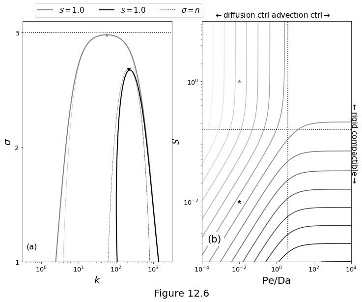
Properties of the dispersion curve near its maximum, with \(n=3,\,\Da=10^4,\,b=\pi\). (a) Comparison of the exact dispersion relation \(\eqref{eq:rxflow-analytical-sigma-full}\) (solid lines) with the asymptotic relations \(\eqref{eq:rxflow-asymptotic-sigma}\)-\(\eqref{eq:rxflow-analytic-real-im-asymptotic_e}\) (dashed lines) for \(\Pe/\Da=10^{-2}\) and two values of \(\stiff\), as given in the legend. (b) Contours of fastest-growing (non-dimensional) wavelength \(\lambda^*\) for a range of \(\stiff\) and \(\Pe\) from equation \(\eqref{eq:rxflow-kstar-full}\). Dotted lines are at \(\Pe/\Da = 4\) and \(\stiff = 1/2\pi\). In both panels, stars indicate the maximum (\(\wavenumber^*,\sigma^*\)) of the asymptotic curves, computed with \(\eqref{eq:rxflow-kstar-full}\) and \(\eqref{eq:rxflow-sstar-full}\).
fig = plt.figure(figsize=(12., 9.))
gs = gridspec.GridSpec(1, 2, width_ratios=[1, 1])

ax0 = plt.subplot(gs[0])

Da = 1e4
k = np.logspace(-1, 4, 10000).astype(np.clongdouble)
n = 3
Pe = Da / 100
S = np.asarray([1.0, 0.01]).astype(np.clongdouble)
l = 1.0

sfull = full_dispersion(k, n, Da, Pe, S[0], l)
sasym = asym_dispersion(k, n, Da, Pe, S[0], l)
smax = asym_maxgrowth(k, n, Da, Pe, S[0], l)
ax0.loglog(
    sfull.k, sfull.s, '-', linewidth=2,
    color=[0.5, 0.5, 0.5], label=r'$\mathcal{S}='+str(np.real(S[0]))+'$'
)
ax0.loglog(
    np.real(k), sasym, '--',
    linewidth=0.5, color=[0.5, 0.5, 0.5]
)
ax0.plot(
    smax.k, smax.s, '*', markersize=7,
    color=[0.5, 0.5, 0.5]
)

sfull = full_dispersion(k, n, Da, Pe, S[1], l)
sasym = asym_dispersion(k, n, Da, Pe, S[1], l)
smax = asym_maxgrowth(k, n, Da, Pe, S[1], l)
ax0.loglog(
    sfull.k, sfull.s, '-k', linewidth=2,
    label=r'$\mathcal{S}='+str(np.real(S[0]))+'$'
)
ax0.loglog(np.real(k), sasym, '--k', linewidth=0.5)
ax0.plot(smax.k, smax.s, '*k', markersize=7)

ax0.plot(
    np.real([k[0], k[-1]]), [n, n], ':k', label=r'$\sigma=n$'
)

ax0.set_xlim(np.sqrt(0.1), np.power(10, 3.5))
ax0.set_xticks([1.e0, 1.e1, 1.e2, 1.e3])
ax0.set_xlabel(r'$k$', fontsize=20)

ax0.set_ylabel(r'$\sigma$', fontsize=20)
ax0.set_ylim(1.0, 3.1)
ax0.set_yscale('linear')
ax0.set_yticks([1, 2, 3])
ax0.tick_params(axis='both', which='major', labelsize=13)

ax0.text(
    0.4, 1.1, r'(a)', fontsize=16,
    verticalalignment='bottom', horizontalalignment='left'
)

ax0.legend(
    fontsize=15, loc='upper left',
    bbox_to_anchor=(0.06, 1.09), ncol=3
)

ax1 = plt.subplot(gs[1])

Spts = S
Pe_Da = Pe / Da

Pe = np.logspace(np.log10(Da) - 4.0, np.log10(Da) + 4, 100)
S = np.logspace(-3.0, 1.0, 100)
X, Y = np.meshgrid(Pe, S)
B = np.pi ** 2 + 1. / (2 * Y) ** 2
Ks = np.power(4 * Da * X * B / (4 + X / Da), 0.25)
lambda_ = 2 * np.pi / Ks

ax1.contour(Pe / Da, S, np.log10(lambda_), 16, cmap='gray')
ax1.plot([Pe[0]/Da, Pe[-1]/Da], [1/2/np.pi, 1/2/np.pi], ':k')
ax1.plot([4, 4], [S[1], S[-1]], ':k')
ax1.plot(Pe_Da, np.real(Spts[0]), '*', markersize=7, color=[0.5, 0.5, 0.5])
ax1.plot(Pe_Da, np.real(Spts[1]), '*k', markersize=7)
ax1.set_xscale('log')
ax1.set_yscale('log')
ax1.set_xticks((1.e-4, 1.e-2, 1.e0, 1.e2, 1.e4))
ax1.set_yticks((1.e-2, 1.e0))
ax1.set_ylabel(r'$\mathcal{S}$', fontsize=20)
ax1.set_xlabel(r'Pe$/$Da', fontsize=20)
ax1.tick_params(axis='both', which='major', labelsize=13)
ax1.text(
    0.0002, 0.002, r'(b)', fontsize=20, verticalalignment='bottom',
    horizontalalignment='left', backgroundcolor='w'
)
ax1.text(
    1.4e4, 0.02, r'$\leftarrow$rigid compactible$\rightarrow$',
    rotation=-90, horizontalalignment='center',
    verticalalignment='bottom', fontsize=15
)
ax1.text(
    0.58, 11, r'$\leftarrow$diffusion ctrl advection ctrl$\rightarrow$',
    horizontalalignment='center', verticalalignment='bottom', fontsize=15
)

fig.supxlabel("Figure 12.6", fontsize=20)

plt.show()
Application to the mantle
Parameters and their values (and ranges) for application to the mantle beneath mid-ocean ridges:
Variable (unit) |
Symbol |
Estimate (range) |
|---|---|---|
Permeability exponent |
\(\permexp\) |
\(3\) \((2-3)\) |
Solubility gradient (m\(^{-1}\)) |
\(\beta\) |
\(2\times10^{-6}\) (\(10^{-6}-4\times10^{-6}\)) |
Compositional offset |
\(\alpha\) |
\(1\) |
Melting region depth (m) |
\(H\) |
\(8\times10^{4}\) |
Compaction length (m) |
\(\cmplength\) |
\(10^{3}\) (\(3\times10^2-10^4\)) |
Melt flux (m s\(^{-1}\)) |
\(\por_0 w_0\) |
\(3\times10^{-11}\) (\(5\times10^{-12}-2\times10^{-10}\)) |
Diffusivity (m\(^2\)s\(^{-1}\)) |
\(\por_0 \chemdiffuse\) |
\(3\times10^{-14}\) (\(10^{-15}-10^{-12}\)) |
Reaction rate (s\(^{-1}\)) |
\(\rxnrate\) |
\(3\times10^{-8}\) (\(10^{-11}-10^{-4}\)) |
Decompression melting rate (s\(^{-1}\)) |
\(W_0\adiprod\) |
\(3\times10^{-15}\) (\(10^{-15} - 10^{-14}\)) |
Melt productivity~ratio |
\(\dpro\) |
\(45\) (\(1-200\)) |
Reactive melt volume |
\(\rpro\) |
\(0.14\) (\(0.07-0.28\)) |
Peclet number |
\(\Pe\) |
\(7\times10^9\) (\(3.5\times10^7 - 1.4\times10^{12}\)) |
Damköhler number |
\(\Da\) |
\(7 \times 10^7\) (\(3.5\times10^3 - 1.4\times10^{12}\)) |
Stiffness number |
\(\stiff\) |
\(3\times10^{-5}\) (\(1\times10^{-6} - 6\times10^{-3}\)) |
class PAR:

    def __init__(self):

        self.n = 3      # permeability exponent
        self.S = 3e-5   # rigidity parameter
        self.Da = 7e7   # Damkohler number
        self.Pe = 7e9   # Peclet number
        self.H = 8e4    # column height, metres
        self.tscale = 1 * 0.01 / 3e-11 / 2e-6 / (np.pi * 1e7)  # years


def Dispersion(k, n, Da, Pe, S):

    k = k.astype(np.clongdouble)
    k2 = k * k
    k4 = k2 * k2
    k6 = k4 * k2
    n, Da, Pe, S = np.clongdouble([n, Da, Pe, S])
    K = 1 + k ** 2 / Da / Pe
    K2 = K * K
    K4 = K2 * K2
    Da2 = Da * Da
    Da3 = Da2 * Da
    Da4 = Da2 * Da2
    b = np.clongdouble(np.pi)
    b2 = b * b
    S2 = S * S
    # upper branch
    s = (2.0 * n * \
        np.sqrt(
            -Da4 * K4 * b2 - Da4 * K4 * k2
            + Da4 * K2 * S2 * k4 - 3.0 * Da3 * K2 * S * k4
            - 2 * Da2 * K2 * b2 * k2 - Da * S * k6 - b2 * k4
        )
        + 4.0 * Da * K * b2 * n + Da * K * k2 * n
        + 2 * Da2 * K * S * k2 * n
    ) / (
        4 * S * Da2 * K2 * b2 + 4.0 * S * Da2 * K2 * k2 + S * k4
    )
    s[np.imag(s) != 0.0] = np.nan
    return np.real(s).astype(np.float32)
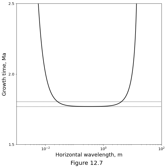
Figure below plots the time-scale of channel growth \(1/\sigma\) as a function of the horizontal wavelength of channels. This curve is computed using the full dispersion relation \(\eqref{eq:rxflow-analytical-sigma-full}\) with preferred parameter values from table above. Horizontal dotted lines mark the minimum growth time (\(\sigma=1/\permexp\), in non-dimensional terms) and this value plus 2%.
fig = plt.figure(figsize=(9., 9.))

par = PAR()
k = np.logspace(4, 8, 10000)
s = Dispersion(k, par.n, par.Da, par.Pe, par.S)

lambda_ = (2 * np.pi / k) * par.H              # metres
tau = (1. / s) * par.tscale / 1e6              # million years
tau_ref = (1. / par.n) * par.tscale / 1e6      # million years
tau_ref90 = (1.02 / par.n) * par.tscale / 1e6  # million years

plt.semilogx(lambda_, tau, '-k', linewidth=2)
plt.plot([1e-5, 1e5], [tau_ref, tau_ref], ':k')
plt.plot([1e-5, 1e5], [tau_ref90, tau_ref90], ':k')
plt.xlim(1e-3, 1e2)
plt.ylim(1.5, 2.5)
plt.xticks((1e-2, 1e0, 1e2))
plt.yticks((1.5, 2.0, 2.5))
plt.xlabel('Horizontal wavelength, m', fontsize=18)
plt.ylabel('Growth time, Ma', fontsize=18)
plt.tick_params(axis='both', which='major', labelsize=13)

fig.supxlabel("Figure 12.7", fontsize=20)

plt.show()